Introduction

Neural Radiance Fields use straightforward volume rendering techniques to avoid the complexities associated with differentiating through ray-triangle intersections, taking advantage of a probabilistic understanding of visibility. This is achieved by assuming that the scene is composed of a spatially varying density of light-emitting particles (in the language of physically-based rendering, this would be described as a volume with absorption and emission, without scattering). For the sake of clarity in the explanation, and without compromising generality, we assume that the emitted light does not change depending on the viewing direction.

Transmittance

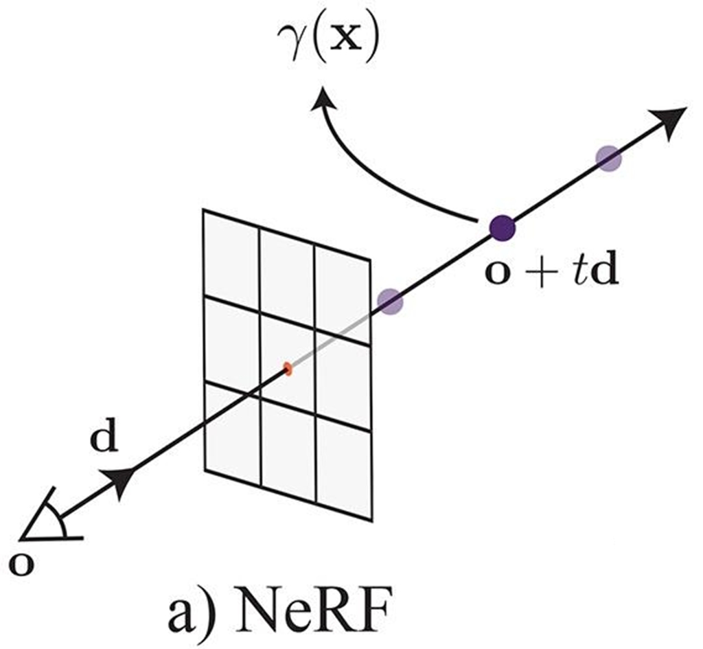
Consider the density field \sigma(x), where x \in \R^3, representing the differential probability of a ray intersecting a particle (i.e., the likelihood of encountering a particle over an infinitesimal distance). We reparameterize the density along a specific ray r=(o, d) as a scalar function \sigma(t), as any point x along the ray can be expressed as r(t)=o+td. Density is intimately linked to the transmittance function \mathcal{T}(t), which denotes the probability of a ray traversing the interval [0, t) without colliding with any particles. Consequently, the probability \mathcal{T}(t+dt) of avoiding a particle when taking a differential step dt is equivalent to \mathcal{T}(t), the probability of the ray reaching t, multiplied by (1 − dt \cdot \sigma(t)), the likelihood of not encountering anything during the step:

\begin{aligned} \mathcal{T}(t+d t) &= \mathcal{T}(t) \cdot(1-d t \cdot \sigma(t)) \\ \frac{\mathcal{T}(t+dt)-\mathcal{T}(t)}{dt} &\equiv \mathcal{T}'(t+dt) = -\mathcal{T}(t) \cdot \sigma(t) \end{aligned}

This is a standard differential equation, the solution to which can be derived as follows:

\begin{aligned} \mathcal{T}^{\prime}(t) & =-\mathcal{T}(t) \cdot \sigma(t) \\ \frac{\mathcal{T}^{\prime}(t)}{\mathcal{T}(t)} & =-\sigma(t) \\ \int_a^b \frac{\mathcal{T}^{\prime}(t)}{\mathcal{T}(t)} d t & =-\int_a^b \sigma(t) d t \\ \left.\log \mathcal{T}(t)\right|_a ^b & =-\int_a^b \sigma(t) d t \\ \mathcal{T}(a \rightarrow b) \equiv \frac{\mathcal{T}(b)}{\mathcal{T}(a)} & =\exp \left(-\int_a^b \sigma(t) d t\right) \end{aligned}

Here, we designate \mathcal{T}(a \rightarrow b) as the likelihood of the ray traversing from the distance a to b along the ray without encountering a particle, which correlates with the previous notation as \mathcal{T}(t)=\mathcal{T}(0 \rightarrow t).

Probabilistic interpretation

Note that we can also interpret the function 1 - \mathcal{T}(t) (commonly referred to as opacity) as a cumulative distribution function (CDF) signifying the probability that the ray does intersect a particle at some point before reaching distance t. Consequently, \mathcal{T}(t) \cdot \sigma(t) represents the corresponding probability density function (PDF), providing the probability that the ray halts exactly at a distance t.

Volume rendering

We are now equipped to compute the expected value of the light emitted by the particles within the volume as the ray progresses from t=0 to D, composited atop a background color. Given that the probability density for halting at t is \mathcal{T}(t) \cdot \sigma(t), the anticipated color is

\boldsymbol{C}=\int_0^D \mathcal{T}(t) \cdot \sigma(t) \cdot \mathbf{c}(t) d t+\mathcal{T}(D) \cdot \mathbf{c}_{\mathrm{bg}}

where \mathbf{c}_{\mathrm{bg}} represents a background color that is composited with the foreground scene in accordance with the remaining transmittance \mathcal{T}(D). For the sake of generality, we will exclude the background term in the subsequent discussion.

Homogeneous media

We can determine the color of certain homogeneous volumetric media with a constant color c_a and density \sigma_a over a ray segment [a, b] through the process of integration:

\begin{aligned}\boldsymbol{C}(a \rightarrow b) & =\int_a^b \mathcal{T}(a \rightarrow t) \cdot \sigma(t) \cdot \mathbf{c}(t) d t \\& =\sigma_a \cdot \mathbf{c}_a \int_a^b \mathcal{T}(a \rightarrow t) d t \\& =\sigma_a \cdot \mathbf{c}_a \int_a^b \exp \left(-\int_a^t \sigma(u) d u\right) d t \\& =\sigma_a \cdot \mathbf{c}_a \int_a^b \exp \left(-\left.\sigma_a u\right|_a ^t\right) d t \\& =\sigma_a \cdot \mathbf{c}_a \int_a^b \exp \left(-\sigma_a(t-a)\right) d t \\& =\left.\sigma_a \cdot \mathbf{c}_a \cdot \frac{\exp \left(-\sigma_a(t-a)\right)}{-\sigma_a}\right|_a ^b \\& =\mathbf{c}_a \cdot\left(1-\exp \left(-\sigma_a(b-a)\right)\right)\end{aligned}

Transmittance is multiplicative

Note that the transmittance can be factorized as follows:

\begin{aligned}\mathcal{T}(a \rightarrow c)= & =\exp \left(-\left[\int_a^b \sigma(t) d t+\int_b^c \sigma(t) d t\right]\right) \\& =\exp \left(-\int_a^b \sigma(t) d t\right) \exp \left(-\int_b^c \sigma(t) d t\right) \\& =\mathcal{T}(a \rightarrow b) \cdot \mathcal{T}(b \rightarrow c)\end{aligned}

This is also a consequence of the probabilistic interpretation of \mathcal{T}, as the likelihood that the ray does not intersect any particles within [a, c] is the product of the probabilities of the two independent events that it does not intersect any particles within [a, b] or within [b, c].

Transmittance for piecewise constant data

Given a set of intervals \{[t_n, t_{n+1}]\}{n=1}^N with a constant density \sigma_n within the n-th segment, and with t_1=0 and \delta_n=t{n+1}−t_n, the transmittance can be expressed as:

\mathcal{T}_n=\mathcal{T}\left(t_n\right)=\mathcal{T}\left(0 \rightarrow t_n\right)=\exp \left(-\int_0^{t_n} \sigma(t) d t\right)=\exp \left(\sum_{k=1}^{n-1}-\sigma_k \delta_k\right)

Volume rendering of piecewise constant data

By integrating the above, we can compute the volume rendering integral through a medium characterized by piecewise constant color and density:

\begin{aligned}\boldsymbol{C}\left(t_{N+1}\right) & =\sum_{n=1}^N \int_{t_n}^{t_{n+1}} \mathcal{T}(t) \cdot \sigma_n \cdot \mathbf{c}n d t \\& =\sum{n=1}^N \int_{t_n}^{t_{n+1}} \mathcal{T}\left(0 \rightarrow t_n\right) \cdot \mathcal{T}\left(t_n \rightarrow t\right) \cdot \sigma_n \cdot \mathbf{c}n d t \\& =\sum{n=1}^N \mathcal{T}\left(0 \rightarrow t_n\right) \int_{t_n}^{t_{n+1}} \mathcal{T}\left(t_n \rightarrow t\right) \cdot \sigma_n \cdot \mathbf{c}n d t \\& =\sum{n=1}^N \mathcal{T}\left(0 \rightarrow t_n\right) \cdot\left(1-\exp \left(-\sigma_n\left(t_{n+1}-t_n\right)\right)\right) \cdot \mathbf{c}_n\end{aligned}

This leads to the volume rendering equations from NeRF [3, Eq.3]:

\boldsymbol{C}\left(t_{N+1}\right)=\sum_{n=1}^N \mathcal{T}_n \cdot\left(1-\exp \left(-\sigma_n \delta_n\right)\right) \cdot \mathbf{c}_n, \quad \text { where } \quad \mathcal{T}n=\exp \left(\sum{k=1}^{n-1}-\sigma_k \delta_k\right)

Ultimately, instead of formulating these expressions in terms of volumetric density, we can recast them in terms of alpha-compositing weights \alpha_n ≡ 1 − \exp(−\sigma_n\delta_n), and by acknowledging that \prod_i \exp x_i = \exp (\sum_i x_i):

\boldsymbol{C}\left(t_{N+1}\right)=\sum_{n=1}^N \mathcal{T}_n \cdot \alpha_n \cdot \mathbf{c}_n, \quad \text { where } \quad \mathcal{T}_n=\prod_{n=1}^{N-1}\left(1-\alpha_n\right)

Alternate derivation

By leveraging the prior relationship between CDF and PDF that (1 - \mathcal{T})' = \mathcal{T} \sigma , and by presuming a constant color c_a along an interval [a, b]:

\begin{aligned}\int_a^b \mathcal{T}(t) \cdot \sigma(t) \cdot \mathbf{c}(t) d t & =\mathbf{c}_a \int_a^b(1-\mathcal{T})^{\prime}(t) d t \\& =\left.\mathbf{c}_a \cdot(1-\mathcal{T}(t))\right|_a ^b \\& =\mathbf{c}_a \cdot(\mathcal{T}(a)-\mathcal{T}(b)) \\& =\mathbf{c}_a \cdot \mathcal{T}(a) \cdot(1-\mathcal{T}(a \rightarrow b))\end{aligned}

When amalgamated with a constant per-interval density, this identity results in the same expression for color as:

\boldsymbol{C}\left(t_{N+1}\right)=\sum_{n=1}^N \mathcal{T}_n \cdot\left(1-\exp \left(-\sigma_n \delta_n\right)\right) \cdot \mathbf{c}_n, \quad \text { where } \quad \mathcal{T}_n=\exp \left(\sum_{k=1}^{n-1}-\sigma_k \delta_k\right)