Why Consider C++/CUDA with PyTorch?

PyTorch, a prominent deep learning framework, is primarily developed in Python. Conversely, C++ and CUDA represent distinct programming languages. An essential question arises: Why would one need C++ or CUDA when working with PyTorch? What advantages do they offer to my PyTorch programs?

The primary motivation behind leveraging C++ and CUDA with PyTorch is performance optimization. If you find that your PyTorch programs are executing at satisfactory speeds, you might not feel the need to explore these extensions. However, there are scenarios where native PyTorch might not offer the desired performance, and that's where the power of C++ and CUDA extensions comes into play.

If you want to explore an example implementation of performance optimization using C++/CUDA for trilinear interpolation, you can find the full source code and project on trilinear-interpolation-cuda.

When Does PyTorch Need a Boost?

Non-Parallel Computation

Most computations in PyTorch are executed in parallel. For instance, during training, instead of processing a single data point, we often batch multiple data points (e.g., a batch of 32) and feed them into the network simultaneously. This parallel processing facilitates efficient backpropagation and training. However, there are specific scenarios where parallelization is not feasible, such as volume rendering. When each ray has a varying number of sample points, parallel processing becomes challenging. One might consider using a 'for loop,' but this approach can be computationally expensive. This is precisely where C++/CUDA extensions can provide a significant speedup.

Sequential Computations in Deep Networks

This is a more straightforward scenario. Imagine a Convolutional Neural Network (CNN) with multiple layers. Each layer takes the output from its preceding layer, processes it, and passes it on. For networks with a moderate number of layers (10-20), this sequential processing is efficient. However, for deeper networks, this method can be suboptimal. With C++/CUDA, we can employ a technique known as "fusion." Instead of processing each layer sequentially, we can "fuse" these operations into a single function. This fusion allows for a single function call, optimizing the computational process, especially for very deep networks. However, it's worth noting that such speed gains are most noticeable for networks with a large number of layers. For shallower networks, native PyTorch's performance is commendable.

Trilinear Interpolation Example

Environment Preparation

# Create a new conda environment named 'cppcuda' with Python version 3.8
conda create -n cppcuda python=3.8

# Activate the newly created 'cppcuda' environment
conda activate cppcuda

# Install PyTorch, torchvision, torchaudio, and specify the CUDA version (11.8) for PyTorch
conda install pytorch torchvision torchaudio pytorch-cuda=11.8 -c pytorch -c nvidia

Edit configurations in c_cpp_properties.json:

{
    "configurations": [
        {
            "name": "Linux",
            "includePath": [
                "${workspaceFolder}/**",
                "/home/user/miniconda3/envs/cppcuda/include/python3.8",
                "/home/user/miniconda3/envs/cppcuda/lib/python3.8/site-packages/torch/include",
                "/home/user/miniconda3/envs/cppcuda/lib/python3.8/site-packages/torch/include/torch/csrc/api/include"
            ],
            "defines": [],
            "compilerPath": "/usr/bin/gcc",
            "cStandard": "c17",
            "cppStandard": "gnu++17",
            "intelliSenseMode": "linux-gcc-x64"
        }
    ],
    "version": 4
}

CUDA Integration

CUDA Execution Function

The foremost responsibility of the C++ layer is to define a function that initiates CUDA execution. This function serves as the entry point for all GPU-related computations that PyTorch aims to perform.

torch::Tensor trilinear_interpolation(
    torch::Tensor feats,
    torch::Tensor points
){
    return feats;
}

Python-C++ Interface

The next crucial step is to establish an interface that allows Python (and by extension, PyTorch) to invoke the C++ function. If you've ventured into the world of interfacing Python with C++ before, you might be familiar with the pybind library.

Understanding the Role of pybind

pybind is a lightweight header-only library designed to expose C++ types in Python and vice versa. Its primary purpose is to create Python bindings for pre-existing C++ code. The goals and syntax of pybind closely mirror those of the renowned Boost.Python library by David Abrahams. The main advantage of using pybind is its ability to minimize boilerplate code in traditional extension modules. It achieves this by inferring type information through compile-time introspection.

In the context of our integration, pybind plays a pivotal role. It serves as the bridge, allowing Python (and by extension, PyTorch) to seamlessly interface with C++ functions. Whether you're working with PyTorch or other frameworks like OpenCV, pybind offers a streamlined approach to meld Python and C++ functionalities.

Setting Up the Interface

Creating this interface is a straightforward process, especially if you have a template or prior work to refer to. Most of the foundational code remains consistent, with only minor modifications needed:

• Function Naming Convention: The string argument in m.def represents the function name as it will be invoked from Python. For consistency and clarity, it's advisable to use the same name as the original C++ function.

• Linking to the C++ Function: The subsequent argument in m.def is a direct reference to the C++ function that will be triggered when the Python call is made.

With these steps completed, our C++ bridge, serving as the conduit between PyTorch and CUDA, is effectively established.

PYBIND11_MODULE(TORCH_EXTENSION_NAME, m){
    m.def("trilinear_interpolation", &trilinear_interpolation);
}

PyTorch C++ Extension Setup

1. Importing Essential Modules

The initial lines of our setup script are dedicated to importing necessary modules. In our case, we're leveraging CppExtension for the C++ integration and BuildExtension for the build process.

from setuptools import setup
from torch.utils.cpp_extension import BuildExtension, CppExtension

2. Configuring the Package Details

Inside the setup function, the first string parameter represents the name of the package. This is the name you'll use when importing the package in Python. For instance, PyTorch is imported using import torch, and TensorFlow with import tensorflow.

setup(
    name='cppcuda',
		version='1.0',
    author='author',
    author_email='author email',
    description='cppcuda example',
    long_description='cppcuda example',
)

Additionally, the setup allows for optional metadata such as the author's name, email, a brief description of the package, and more. While these details are optional, they are beneficial for documentation and distribution purposes.

3. Specifying Source Files

One of the most critical components of the setup is specifying the source files for the extension. This is done using the sources parameter. For example, if our extension is based on the file interpolation.cpp, we would specify it as follows:

ext_modules=[
        CUDAExtension(
            name='cppcuda',
            sources=['interpolation.cpp']
        )
    ]

If your extension comprises multiple source files, simply expand the list by adding the filenames, separated by commas.

4. Command Class Configuration

The final piece of the puzzle is the cmdclass parameter. This tells the setup that we're building the specified C++ code. It's a directive to ensure the correct build process is initiated for our extension.

cmdclass={'build_ext':BuildExtension}

PxTorch C++ Extension Build

1. Initiating the Build Process

To kickstart the build, use the pip install command. The target of this command is the directory containing the setup.py file. If your setup.py is located in the current directory, you can reference it using the . notation:

pip install .

2. Building Duration

While the build process is generally efficient, the duration can vary based on the number and complexity of the source files. In our case, since we're working with a single file, the build should be completed relatively quickly.

Parallel Computing

Parallelism is at the heart of GPU computing, and NVIDIA's CUDA platform offers a robust framework to harness this power. Let's explore the intricate architecture of CUDA and understand how it achieves unparalleled parallelism.

CUDA Basics

The CUDA Architecture: Host vs. Device

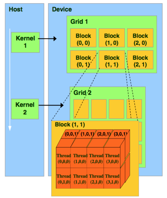
In the CUDA ecosystem, computations are divided between the "host" (CPU) and the "device" (GPU). An illustrative graph detailing this division can be found here. When a function from the host (our C++ program) invokes a CUDA function, several processes are set into motion:

1. Kernel Instantiation: Each CUDA function call from the host initiates a "kernel" on the device. This kernel is responsible for managing the GPU computations.

2. Data Transfer: The data required for computation is transferred from the host (CPU) to the device (GPU).

3. Grid Generation: Alongside data transfer, a "grid" is generated on the device. This grid is the primary structure responsible for parallel computation.

Deciphering the Grid: Blocks and Threads

The grid is a hierarchical structure comprising multiple computational units:

• Blocks: The grid is divided into "blocks." The number of blocks can be programmatically determined. Each block can be further subdivided.

• Threads: Each block contains multiple "threads," which are the fundamental units of computation in CUDA. When a function is invoked, it instantiates a grid with numerous blocks, each containing multiple threads. These threads operate in parallel, enhancing computational throughput.

For instance, consider a matrix addition operation. The program might generate a grid with as many threads as there are matrix elements. Each thread then performs the addition of two corresponding matrix elements.

Why Blocks? Why Not Just Threads?

A pertinent question arises: Why introduce the concept of blocks? Why not have a grid with just threads? The answer lies in hardware limitations. Each block can contain a maximum of 1024 threads due to hardware constraints. However, the number of blocks is significantly larger, with an upper limit of(2^{31}-1) \times 2^{16} \times 2^{16}. By introducing blocks, CUDA effectively increases the total number of threads that can operate in parallel, thereby maximizing computational power.

Achieving Parallelism: The Power of Minimal Work Units

The essence of CUDA's efficiency lies in its ability to distribute minimal work units across a vast number of threads. For example, a simple operation like adding two numbers is distributed across multiple threads, each operating on different data points. This distribution ensures that each thread, or "worker," performs a task requiring roughly the same computational resources and time. By dividing the overall task into such sub-tasks, CUDA accelerates the entire process, achieving high throughput.

Trilinear Interpolation Fundamentals

Understanding Bilinear Interpolation: A Prelude to Trilinear Interpolation

Explaining trilinear interpolation directly in a 3D context can be intricate. To simplify, let's first explore its 2D counterpart: bilinear interpolation. The transition from 2D to 3D will then become intuitive.

• Bilinear vs. Trilinear: The terms "bi" and "tri" refer to the dimensions involved. In 2D (bilinear), we deal with squares, while in 3D (trilinear), we work with cubes.

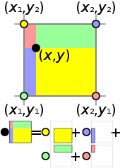
• Interpolation in 2D: Consider a square where each vertex possesses a feature vector. Our objective is to compute the feature of a point inside the square, interpolated from the vertex features. If we denote this feature asf, it becomes a function off_1,f_2,f_3, andf_4.

• Normalization and Weighted Averages: To computef, we first normalize the square's side length to 1. The featuref is then a weighted average of the vertex features, with weights determined by distances to the sides. Let's denote the distance to the left side asu and to the upper side asv. The complementary distances are1-u and1-v.

• Weight Calculation: The weight of each feature is the product of the distances to the opposite sides. For instance, the weight off_1 is(1-u)(1-v). This ensures that in scenarios where the point coincides with a vertex, the weight assigned to that vertex's feature is 1.

Extending to Trilinear Interpolation

Building on our understanding of bilinear interpolation, we can extend the concept to 3D:

• Introducing a Third Dimension: In 3D, we introduce an additional parameter,w, representing the distance to the z-axis. Thus, we haveu,v, andw corresponding to distances to the x, y, and z axes, respectively.

• Weighted Averages in 3D: The weighted average in 3D involves coefficients like uvw,(1-u)vw, etc., multiplied by the features on the opposite sides of the cube.

Designing a CUDA Trilinear Interpolation Program

Understanding Input Tensors

From our previous discussions, we've identified two primary inputs:

1. Vertex Features (feats): This tensor represents the features of the vertices. Its shape is defined as(N, 8, F), where:

   • N represents the number of cubes.

   • The number 8 signifies the vertices of a cube.

   • F denotes the number of features associated with each vertex.

2. Point Coordinates (points): This tensor captures the local coordinates of the points we aim to interpolate. Its shape is(N,3), where:

   • N is the number of points.

   • Each point corresponds to a cube in the feats tensor, ensuring that their first dimensions are congruent.

Strategizing Parallelization

Given the shapes of our tensors, we can identify potential avenues for parallelization:

1. Parallelizing Points: Since the interpolation of each point is independent of others, we can parallelize across theN points. This approach leverages the inherent parallelism of GPUs to compute interpolations for multiple points simultaneously.

2. Parallelizing Features: Similarly, when dealing with multiple features, the interpolation of one feature is agnostic to others. This independence allows us to parallelize across theF features, further enhancing computational efficiency.

Transitioning from C++ to CUDA

1. Understanding the Input Tensors

Our primary function, trilinear_interpolation, returns its first input. To transition this function to CUDA, we'll need to:

• Create a new CUDA file, named interpolation_kernel.cu. The .cu extension signifies CUDA code.

• Define the function prototype within this file. For clarity, we'll rename it to trilinear_fw_cu. The suffixes fw and cu denote "forward pass" and "CUDA code" respectively.

torch::Tensor trilinear_fw_cu(
    torch::Tensor feats,
    torch::Tensor points
){
    return feats;
}

2. Integrating CUDA with C++

To ensure seamless integration:

• Declare the CUDA function within the C++ environment. This can be achieved by creating a header file (often named utils.h) within an include folder.

• This header file should contain the function declaration, ensuring C++ recognizes its existence.

• In the primary C++ file, include the aforementioned header.

3. Ensuring Input Integrity with Macros:

Before diving into the CUDA code, it's imperative to validate our inputs. This is where our "magic" macros come into play:

• CHECK_CUDA: Validates if a tensor resides on CUDA. For computations on CUDA, tensors must be transferred from the CPU.

• CHECK_CONTIGUOUS: Ensures that a tensor's storage remains consistent post-flattening. This is crucial for parallel computation, where memory positions must be continuous.

• CHECK_INPUT: A composite check that validates both the above conditions.

To utilize these checks, simply include the macros in the header and invoke CHECK_INPUT on each tensor before passing it to CUDA.

#define CHECK_CUDA(x) TORCH_CHECK(x.is_cuda(), #x " must be a CUDA tensor")
#define CHECK_CONTIGUOUS(x) TORCH_CHECK(x.is_contiguous(), #x " must be contiguous")
#define CHECK_INPUT(x) CHECK_CUDA(x); CHECK_CONTIGUOUS(x)

Integrating CUDA into C++ Projects

1. Transitioning from CppExtension to CUDAExtension

In our previous setup, we utilized CppExtension. However, with our shift towards CUDA, it's essential to transition to CUDAExtension. This change signifies that our project is now CUDA-ready and can harness the power of GPU acceleration.

from torch.utils.cpp_extension import CUDAExtension

2. Streamlining Source File Inclusion with glob

Manually listing every source file can be tedious and error-prone, especially as the project grows. To automate this process, we can leverage Python's native glob package. With glob, we can:

• Retrieve all .cpp files: glob.glob('*.cpp')

• Fetch all .cu (CUDA) files: glob.glob('*.cu')

By consolidating these lists, we ensure that all relevant source files are included without the risk of omissions or typos.

sources = glob.glob('*.cpp')+glob.glob('*.cu')

3. Specifying Header File Locations

Given the introduction of our utils.h header, it's crucial to inform setup.py of its location. Typically, this header resides within an include directory in the project folder. By specifying this path, we ensure that the setup process recognizes and incorporates the necessary header files.

include_dirs = [osp.join(ROOT_DIR, "include")]

4. Code Optimization with extra_compiler_args

While our primary focus is on functionality, it's worth noting the extra_compiler_args parameter. This pertains to code optimization, aiming to reduce the compiled file size. It's essential to understand that this optimization doesn't enhance the program's speed but focuses solely on file size reduction. Depending on your project's requirements, this step might be optional.

extra_compile_args={'cxx':['-O2'],
                    'nvcc':['-O2']}

5. Final Thoughts

The cmd_class remains consistent with our previous setup. With these modifications in place, your project is now primed to harness the power of CUDA. For future projects, consider using this guide as a template—simply copy the setup and adjust the package names.

Implementing Parallel Computation with CUDA

1. Setting Up the Output Tensor:

Our initial step is to replace the placeholder with the appropriate output tensor. This tensor will serve as the foundation upon which we'll build our computations. To do this:

• Determine the Shape of Tensors: The shape of our tensors is pivotal. In our previous session, we outlined the input tensor shapes. For our output tensor, given that we haveN points and each point hasF features, the shape will be(N,F).

• Generate the Output Placeholder: We can initiate this tensor with any values (zeros, ones, etc.), as we'll be updating these values later. The crucial aspect is to ensure the tensor has the correct shape.

• Extracting Dimensions: Using the C++ API, we can extract the dimensionsN andF from our input tensors. For a comprehensive understanding of the C++ API, refer to the official PyTorch documentation.

• Creating the Output Tensor: With the dimensions in hand, we can now create our output tensor. This tensor should be on the same device as our input tensor and have the same data type. The .options() function in C++ ensures both these conditions are met.

2. Advanced Tensor Creation

Sometimes, our output tensor might require a different data type than our input. In such cases:

• Specify Data Type: Using torch::dtype(), we can set the desired data type for our tensor. For instance, for a 32-bit integer, we'd use torch::kInt32.

• Set Device: The .device() function ensures our tensor is on the correct device. To match the device of our feats tensor, we'd use feats.device().

const int N = feats.size(0), F = feats.size(2);
torch::Tensor feat_interp = torch::zeros({N, F}, feats.options());

3. Determining Block and Thread Sizes

Threads: The primary focus is on determining the number of threads per block. Considering our algorithm, we identified two dimensions for parallel computation:N points andF features. The rule of thumb is to set the total number of threads to 256, distributing them evenly across the dimensions. However, this number is not set in stone and can be adjusted based on the specific requirements of the algorithm and hardware.

Blocks: The number of blocks is deduced from a formula based on the shape of the inputs and the size of the threads. The principle is to ensure that the blocks, when multiplied by the thread size, cover the entire data set. For instance, if we haveN=20 data points and threads.x=16, we would need 2 blocks along one dimension to cover all data points. The formula for this is:

const dim3 threads(16, 16);  // 256=16*16 threads
const dim3 blocks((N+threads.x-1)/threads.x, (F+threads.y-1)/threads.y);

4. Kernel Launching

Kernel launching is the process of initiating the parallel computation on the GPU. The syntax remains consistent, with only the arguments changing based on the specific function. The function AT_DISPATCH_FLOATING_TYPES is pivotal here, as it determines the type of floating operations the kernel will perform, be it float32 or float64 for optimized performance.

5. Practical Tips for Kernel Launching

• Function Naming: It's advisable to keep the kernel function name consistent with the CUDA function name. This ensures clarity and aids in debugging, as any errors thrown will reference this name.

• Data Type Consistency: Ensure that the data type you're operating on is consistent. For instance, if "feats" is float32, the kernel should perform float32 operations.

• Error Handling: Proper error handling mechanisms should be in place. If a kernel launch fails, the system should throw an error with the function's name, allowing for quick identification and resolution.

6. Understanding Kernel Arguments

Upon a cursory glance, one might be overwhelmed by the plethora of arguments following the kernel name. Let's demystify them:

• Kernel Name: This specifies the kernel function that will be executed. The function contains the logic for the computations we wish to perform in parallel.

• Template for Data Type: This is a flexible way to handle different data types. For instance, FLOATING_TYPES can handle both float32 and float64. By using the scalar_t template, the kernel can automatically infer the data type from the inputs.

• Number of Blocks and Threads: These are specified using the dim3 type (or int). They determine the granularity of parallelism.

• Inputs and Outputs: Unlike traditional functions that return a value, kernels don't return anything. Instead, they modify the output tensor directly. Therefore, both input and output tensors are passed as arguments to the kernel.

7. The Role of Packed Accessor

A unique aspect of CUDA programming is the .packed_accessor method. Since CUDA doesn't inherently recognize the "tensor" type, this method converts tensors into a type that CUDA understands, called "PackedAccessor". This conversion is essential for manipulating tensors within the kernel.

The arguments following .packed_accessor serve specific purposes:

• Data Type: By setting scalar_t, the kernel can handle any type of floating numbers. If the data type is known in advance, it can be explicitly set, providing more control but potentially reducing flexibility.

• Number of Dimensions: This specifies the tensor's dimensionality. For instance, a tensor with shape (N, 8, F) would have a dimensionality of 3.

• RestrictPtrTraits: This ensures that the tensor doesn't overlap with other tensors in memory.

• Size_t: This specifies the data type used for tensor indices. Typically, it's best to leave this as size_t.

8. Flexibility vs. Specificity

While the use of scalar_t offers flexibility, allowing the kernel to handle various data types, there might be scenarios where a specific data type is required. In such cases, the data type can be explicitly set, ensuring that the kernel operates only on tensors of that particular type.

AT_DISPATCH_FLOATING_TYPES(feats.type(), "trilinear_fw_cu", 
    ([&] {
        trilinear_fw_kernel<scalar_t><<<blocks, threads>>>(
            feats.packed_accessor<scalar_t, 3, torch::RestrictPtrTraits, size_t>(),
            points.packed_accessor<scalar_t, 2, torch::RestrictPtrTraits, size_t>(),
            feat_interp.packed_accessor<scalar_t, 2, torch::RestrictPtrTraits, size_t>()
        );
    }));

return feat_interp;

9. Function Signatures in CUDA

The function definition in CUDA has some unique characteristics:

• global Keyword: This keyword signifies that the function is invoked by the host (CPU) but executed on the GPU. In essence, when you call the kernel using "AT_DISPATCH", the __global__ keyword is mandatory, indicating the function's execution on the GPU.

• Return Type: Unlike traditional functions, kernels don't return values. Instead, they modify the output tensor directly. Thus, the return type is always void.

• Function Name: This is the identifier for the kernel and is essential for its invocation.

10. Other CUDA Keywords

Apart from __global__, CUDA offers other keywords to specify where the function is called and executed:

• __**host__**: As the name suggests, this keyword indicates that the function is both called and executed on the CPU.

• __**device__**: Contrary to __host__, this keyword denotes that the function is both called and executed on the GPU. It's primarily used for functions invoked from within the kernel.

11. Understanding Packed Accessors

The inputs to our kernel are packed accessors, which we previously converted. These are data types under the Torch namespace, and their arguments remain consistent with our prior discussion. An optimization tip: use the const keyword for inputs that remain unchanged, ensuring efficiency.

12. Kernel Execution and Parallelism

The heart of parallel computing lies in the kernel's execution. Each thread in the kernel is responsible for computing a specific element of the output tensor. The process is as follows:

1. Compute the ID for Each Thread: Each thread has a unique global ID, calculated based on its position within the block and its local ID.

2. Exclude Redundant Threads: Not all threads will have relevant computations. Some might be redundant, and it's crucial to exclude them to prevent unnecessary operations and potential memory leaks.

3. Parallel Computation: Each thread performs its designated computation. For instance, in our interpolation example, each thread calculates for a single point and feature based on a pre-defined algorithm.

template <typename scalar_t>
__global__ void trilinear_fw_kernel(
    const torch::PackedTensorAccessor<scalar_t, 3, torch::RestrictPtrTraits, size_t> feats,
    const torch::PackedTensorAccessor<scalar_t, 2, torch::RestrictPtrTraits, size_t> points,
    torch::PackedTensorAccessor<scalar_t, 2, torch::RestrictPtrTraits, size_t> feat_interp
){
    const int n = blockIdx.x * blockDim.x + threadIdx.x;
    const int f = blockIdx.y * blockDim.y + threadIdx.y;

    if (n>=feats.size(0) || f>=feats.size(2)) return;

    // point -1~1
    const scalar_t u = (points[n][0]+1)/2;
    const scalar_t v = (points[n][1]+1)/2;
    const scalar_t w = (points[n][2]+1)/2;
    
    const scalar_t a = (1-v)*(1-w);
    const scalar_t b = (1-v)*w;
    const scalar_t c = v*(1-w);
    const scalar_t d = 1-a-b-c;
    feat_interp[n][f] = (1-u)*(a*feats[n][0][f] +
                               b*feats[n][1][f] +
                               c*feats[n][2][f] +
                               d*feats[n][3][f]) + 
                            u*(a*feats[n][4][f] +
                               b*feats[n][5][f] +
                               c*feats[n][6][f] +
                               d*feats[n][7][f]);
}

Performance Analysis

Verifying CUDA Functionality

1. Setting Up the Environment

   • We begin by generating random inputs for our function. For instance, with N=65536 representing the number of points and F=256 denoting feature length, we can create a tensor feats of shape (N, 8, F) , and a tensor points of shape (N, 3) within the range [-1,1] .

   • It's crucial to set the device to CUDA. Remember, if the tensor remains on the CPU, the function will return an error.

   N = 65536; F = 256
   feats = torch.rand(N, 8, F, device='cuda')
   point = torch.rand(N, 3, device='cuda')*2-1
   

2. Invoking the CUDA Function

   • Import the necessary package, as defined in setup.py.

   • Once imported, all functions defined within the PYBIND_MODULE in .cpp become accessible.

   • By passing the appropriate arguments, we can retrieve the output from the CUDA function and verify its shape. For our trilinear interpolation example, the expected output shape is (N, F).

   out_cuda = cppcuda.trilinear_interpolation(feats, point)
   

Comparative Analysis: CUDA vs. PyTorch

1. PyTorch Counterpart

   • To validate the CUDA function's output, we need a PyTorch version of the same operation. The essence of the operation involves calculating distances to axes and then performing a weighted average of the features.

   • With PyTorch's vectorization capabilities, this becomes a straightforward task.

   def trilinear_interpolation_py(feats, points):
       """
       Inputs:
           feats: (N, 8, F)
           points: (N, 3) local coordinates in [-1, 1]
       
       Outputs:
           feats_interp: (N, F)
       """
       u = (points[:, 0:1]+1)/2
       v = (points[:, 1:2]+1)/2
       w = (points[:, 2:3]+1)/2
       a = (1-v)*(1-w)
       b = (1-v)*w
       c = v*(1-w)
       d = 1-a-b-c
   
       feats_interp = (1-u)*(a*feats[:, 0] +
                             b*feats[:, 1] +
                             c*feats[:, 2] +
                             d*feats[:, 3]) + \\
                          u*(a*feats[:, 4] +
                             b*feats[:, 5] +
                             c*feats[:, 6] +
                             d*feats[:, 7])
       
       return feats_interp
   

2. Output Verification

   • With both out_cuda (from the CUDA kernel) and out_py (from the PyTorch code) in hand, we can employ PyTorch's allclose function. This function checks if two tensors are close within a specified error bound, considering both relative and absolute errors.

   print(torch.allclose(out_cuda, out_py))
   

3. Performance Metrics

   • The primary allure of CUDA is its potential speed advantage. By comparing the runtime of both functions, we can ascertain CUDA's efficiency.

   • Preliminary tests indicate that the CUDA function is slightly faster. However, for a comprehensive analysis, multiple runs and average calculations are recommended.

   t = time.time()
   out_cuda = cppcuda.trilinear_interpolation(feats, point)
   torch.cuda.synchronize()
   print('cuda time: ', time.time()-t)
   
   t = time.time()
   out_py = trilinear_interpolation_py(feats, point)
   torch.cuda.synchronize()
   print('pytorch time: ', time.time()-t)
   

Backpropagation

Backpropagation Overview

Backpropagation is a foundational concept in neural networks, responsible for updating the weights of the network based on the error of the output. In our previous discussion, we delved into the forward pass, particularly focusing on the trilinear interpolation. However, without the ability to compute the backward pass, optimizing our model based on a loss function becomes unattainable. This article aims to elucidate the process of implementing the backward pass in CUDA, ensuring the correct gradient computation for feature updates.

Partial Derivatives

Identifying Trainable Inputs

Before diving into the computation, it's crucial to identify which variables in our function are trainable. This distinction is vital because:

1. It saves significant time by avoiding unnecessary derivative calculations.

2. It ensures the accuracy of the gradient, as missing out on any derivative can lead to incorrect training results.

Using the trilinear interpolation as an example, our output is the interpolated featuref. The inputs to this function areu,v andf_1 tof_4. Among these, onlyf_1 tof_4 are considered trainable in our scenario.

Computing the Derivatives

Given the simplicity of our function, which is primarily a linear combination, we can manually compute the partial derivatives. For more complex functions, one might consider using mathematical software or online calculators. For our function:

Chain Rule & Gradient Computation

To compute the gradient for backpropagation, we employ the chain rule from calculus. Imagining a loss functionL that depends on our interpolated featuref, our goal is to compute the derivatives\frac{dL}{df_1} to\frac{dL}{df_4} .

Using the chain rule:

Here,\frac{dL}{df} is a known value, typically provided by the subsequent layers during backpropagation. By multiplying this with our previously computed partial derivatives, we can obtain the gradients needed for updating our features.

Implementing Backpropagation Algorithm

Setting Up the Backward Pass

1. Initializing the Backward Function

Switch to the interpolation.cu file. The process begins by adapting the forward pass function for the backward pass. Here's a step-by-step guide:

• Copy the forward pass function.

• Rename the function from "fw" to "bw".

• Adjust the function arguments to include\frac{dL}{df}, which represents the gradient of the loss with respect to the interpolated feature.

• The output of this function will be\frac{dL}{dfeats}, encompassing all the gradients\frac{dL}{df_i} fori=1 to 4.

torch::Tensor trilinear_bw_cu(
    const torch::Tensor dL_dfeat_interp,
    const torch::Tensor feats,
    const torch::Tensor points
){
    const int N = feats.size(0), F = feats.size(2);
    
    torch::Tensor dL_dfeats = torch::empty({N, 8, F}, feats.options());

    const dim3 threads(16, 16);
    const dim3 blocks((N+threads.x-1)/threads.x, (F+threads.y-1)/threads.y);

    AT_DISPATCH_FLOATING_TYPES(feats.type(), "trilinear_bw_cu", 
    ([&] {
        trilinear_bw_kernel<scalar_t><<<blocks, threads>>>(
            dL_dfeat_interp.packed_accessor<scalar_t, 2, torch::RestrictPtrTraits, size_t>(),
            feats.packed_accessor<scalar_t, 3, torch::RestrictPtrTraits, size_t>(),
            points.packed_accessor<scalar_t, 2, torch::RestrictPtrTraits, size_t>(),
            dL_dfeats.packed_accessor<scalar_t, 3, torch::RestrictPtrTraits, size_t>()
        );
    }));

    return dL_dfeats;
}

2. Kernel Adjustments

The kernel function, which is executed on the GPU, needs modifications to compute the backward pass:

• Rename the kernel function to bw_kernel.

• Adjust the kernel arguments to include\frac{dL}{df_{interp}} and\frac{dL}{dfeats}.

• Remove the interpolation logic from the forward pass.

• Implement the gradient computation logic using the chain rule.

For instance, the gradient for the first component is computed as:

\frac{dL}{df_1} = \frac{dL}{df} \times (1-u) \times a

Wherea is the coefficient representing(1-v)(1-w) in the 3D example.

const scalar_t u = (points[n][0]+1)/2;
const scalar_t v = (points[n][1]+1)/2;
const scalar_t w = (points[n][2]+1)/2;

const scalar_t a = (1-v)*(1-w);
const scalar_t b = (1-v)*w;
const scalar_t c = v*(1-w);
const scalar_t d = 1-a-b-c;

dL_dfeats[n][0][f] = (1-u)*a*dL_dfeat_interp[n][f];
dL_dfeats[n][1][f] = (1-u)*b*dL_dfeat_interp[n][f];
dL_dfeats[n][2][f] = (1-u)*c*dL_dfeat_interp[n][f];
dL_dfeats[n][3][f] = (1-u)*d*dL_dfeat_interp[n][f];
dL_dfeats[n][4][f] = u*a*dL_dfeat_interp[n][f];
dL_dfeats[n][5][f] = u*b*dL_dfeat_interp[n][f];
dL_dfeats[n][6][f] = u*c*dL_dfeat_interp[n][f];
dL_dfeats[n][7][f] = u*d*dL_dfeat_interp[n][f];

Implementation Insights

1. Tensor Shapes: Always ensure that the shape of a tensor and its gradient are identical. This consistency is crucial for correct gradient propagation.

2. Chain Rule: The chain rule is the backbone of backpropagation. For our trilinear interpolation, each gradient component is computed as the product of\frac{dL}{df} and the corresponding interpolation coefficient.

3. Code Structure: A significant portion of the backward pass implementation involves copying the forward pass and making necessary modifications. This approach simplifies the coding process and ensures consistency.

Integrating with PyTorch

Once the CUDA implementation is complete, the next step is to integrate it with PyTorch:

• Add the backward function to the .cpp and .h files.

• Ensure that the function checks if the tensors are on the CUDA device.

• Update the Python bindings to include the new function.

• Rebuild the library using pip install.

Validating the Backpropagation Implementation

Wrapping CUDA Functions in PyTorch

1. Utilizing torch.autograd.Function:

To seamlessly integrate CUDA functions into PyTorch, we employ the torch.autograd.Function class. This class allows us to wrap both forward (fw) and backward (bw) passes, ensuring that PyTorch can compute gradients during the training process.

2. Defining the Custom Function:

Begin by creating a class that inherits from torch.autograd.Function. This class should implement two primary methods: forward and backward.

• Forward Method: This method computes the forward pass. It accepts an additional argument, ctx, which stands for context. This context is essential as it stores variables required for the backward pass. After computing the forward pass, save any necessary variables using ctx.save_for_backward.

• Backward Method: This method computes the backward pass. It takes the ctx argument, followed by the gradient of the loss with respect to the output. Using the chain rule, compute the gradient of the loss with respect to each input.

class Trilinear_interpolation_cuda(torch.autograd.Function):
    @staticmethod
    def forward(ctx, feats, points):
        feat_interp = cppcuda.trilinear_interpolation_fw(feats, points)

        ctx.save_for_backward(feats, points)

        return feat_interp

    @staticmethod
    def backward(ctx, dL_dfeat_interp):
        feats, points = ctx.saved_tensors

        dL_dfeats = cppcuda.trilinear_interpolation_bw(dL_dfeat_interp.contiguous(), feats, points)

        return dL_dfeats, None

Testing the Implementation

1. Setting Up the Test

To validate the CUDA implementation, we'll compare its results with a native PyTorch implementation. Start by duplicating the input tensors. One will be processed using the PyTorch function, and the other with the CUDA function.

2. Computing the Loss

For this demonstration, let's consider a simple loss function: the sum of the features. By invoking loss.backward(), PyTorch computes the gradients for all tensors involved in the loss computation.

3. Comparing Gradients

After computing the backward pass for both implementations, compare the gradients. If they match, it's an indication that the CUDA implementation is correct.

4. Performance Benchmarking

To ascertain the efficiency of the CUDA implementation, measure the execution time for both forward and backward passes. Compare these timings with the native PyTorch implementation to gauge performance improvements.

• The efficiency of CUDA is further emphasized when examining the backward pass computations. The speed advantage becomes more pronounced in this phase.

• Initial results show that the CUDA backward pass is significantly faster than its PyTorch counterpart. To ensure the robustness of these findings, it's advisable to conduct repeated tests and compute average runtimes.

N = 65536; F = 256
rand = torch.rand(N, 8, F, device='cuda')
feats = rand.clone().requires_grad_()
feats2 = rand.clone().requires_grad_()
point = torch.rand(N, 3, device='cuda')*2-1

t = time.time()
out_cuda = Trilinear_interpolation_cuda.apply(feats2, point)
torch.cuda.synchronize()
print('cuda fw time: ', time.time()-t, 's')

t = time.time()
out_py = trilinear_interpolation_py(feats, point)
torch.cuda.synchronize()
print('pytorch fw time: ', time.time()-t, 's')

print('fw all close', torch.allclose(out_cuda, out_py))

t = time.time()
loss2 = out_cuda.sum()
loss2.backward()
torch.cuda.synchronize()
print('cuda bw time', time.time()-t, 's')

t = time.time()
loss = out_py.sum()
loss.backward()
torch.cuda.synchronize()
print('pytorch bw time', time.time()-t, 's')

print('bw all close', torch.allclose(feats.grad, feats2.grad))

Conclusion

In this comprehensive exploration, we delved into the intricacies of integrating CUDA functions within the PyTorch framework, emphasizing the significance of trilinear interpolation in the context of deep learning applications. The primary motivation behind this endeavor was to harness the computational prowess of CUDA to potentially expedite operations, especially in the realm of forward and backward passes.

Our systematic approach began with setting up the environment, ensuring the correct tensor shapes and device allocations. This was followed by a meticulous process of wrapping the CUDA functions within PyTorch, a step crucial for seamless integration and facilitating both forward and backward operations. The subsequent phase involved rigorous testing of the implementation, which not only validated the correctness of the output but also provided insights into performance metrics.

The performance analysis revealed promising results. Preliminary tests consistently indicated that CUDA functions, both in forward and backward passes, outperformed their PyTorch counterparts in terms of execution speed. Such findings underscore the potential benefits of CUDA, especially in scenarios where computational efficiency is paramount.

However, it's worth noting that while our tests showcased the advantages of CUDA, the real-world applicability might vary based on specific use cases, data sizes, and hardware configurations. It's always recommended to conduct extensive tests tailored to individual project requirements.

In conclusion, the integration of CUDA within PyTorch offers a promising avenue for researchers and practitioners aiming to optimize their deep learning workflows. While the initial setup and integration might seem intricate, the potential gains in computational efficiency make the endeavor worthwhile. As the field of deep learning continues to evolve, such optimizations will play a pivotal role in addressing complex challenges and pushing the boundaries of what's achievable.