Introduction

Kolmogorov-Arnold Networks (KANs) are gaining significant attention within the AI community due to growing dissatisfaction with the foundational module of deep learning networks: Multilayer Perceptrons (MLPs). The rise of large-scale models relying on MLPs has spotlighted several fundamental issues within this architecture. So, what makes KANs stand out? What specific improvements do they offer over MLPs? What are the core principles of KANs that are generating such enthusiasm? We'll explore the advantages of KANs, assess whether they are worth investing in, and discuss how KANs could potentially revolutionize the entire structure of current deep learning paradigms. Let's dive into the transformative potential of KANs in reshaping the landscape of neural network architecture.

Understanding the Essence of MLP

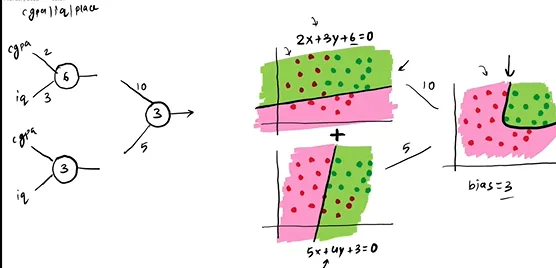
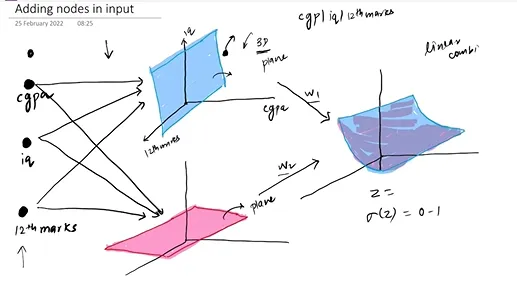
The essence of the Multilayer Perceptrons (MLPs) lies in its utilization of a linear model encapsulated within a nonlinear activation function to facilitate nonlinear space transformations. The primary advantage of a linear model is its simplicity, with each edge represented by two parameters, w and b, which are combined into a matrix vector W. This structure allows for straightforward computation and implementation.

For example, by combining two linear decision boundaries and applying an activation function in the second layer, a nonlinear decision boundary is formed. The two linear decision boundaries, each represented by a straight line, are 2x + 3y + 6 = 0 and 5x + 3y = 0. These lines divide the two-dimensional space into different regions. The output from the first layer typically serves as the input for the second layer, which is then processed through the activation function, creating a complex, nonlinear decision boundary. This transformation occurs because the output of each linear model is influenced by the nonlinear activation function, enabling the model to capture intricate data patterns. The multilayer structure, combined with nonlinear activation functions, allows the network to evolve simple linear decision boundaries through composition and transformation, resulting in nonlinear decision boundaries that can address complex classification problems.

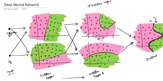
Theoretically, a single hidden layer network with a sufficient number of neurons can approximate any continuous function, as guaranteed by the universal approximation theorem. For instance, a classification boundary can transform into a curved surface, illustrating the power of neural networks to model complex, nonlinear relationships within data.

In MLPs, each layer performs a linear transformation followed by a nonlinear operation. This hierarchical structure enables the model to learn multi-level feature representations of the data. As the number of layers increases, the model's representational capacity also enhances. This is fundamentally why deep learning is effective—the greater the depth, the more powerful the model becomes.

Expressed in the matrix form of linear algebra, it is represented by the following formula:

In this expression, the circle \circ denotes function composition, signifying the combination of multiple functions.

Note: In this context, all activation functions are simplified by using a single type wherever possible. However, there are instances where two different activation functions are employed.

Why do neural networks often use the MLP structure? The simplicity and effectiveness of MLP align with the principle of Occam's Razor. The MLP form is well-suited for understanding fundamental forward and backward propagation algorithms and is straightforward to implement using various programming languages and frameworks. Consequently, it was historically chosen as the foundation of deep learning.

Inherent Flaws of MLP: Is the Current Deep Learning Framework Fragile?

The Multilayer Perceptrons (MLPs), or fully connected network, are widely regarded as the foundation of deep learning. All subsequent network architectures, including Convolutional Neural Networks (CNNs), Recurrent Neural Networks (RNNs), and Transformers, are modifications derived from the MLP framework, even the currently popular large models. However, this foundational module is inherently flawed.

Key Issues with MLPs:

1. Gradient Vanishing and Gradient Explosion: Traditional activation functions, like Sigmoid or Tanh, make MLPs susceptible to gradient vanishing or explosion during backpropagation. This occurs due to successive multiplication of the activation function's derivatives. When these derivatives are very small or very large, especially in deep networks, the gradients can either approach zero (vanishing) or become excessively large (explosion). Both scenarios significantly hinder learning, either stalling weight updates or causing instability.

2. Low Parameter Efficiency: MLPs use fully connected layers, where each neuron connects to all neurons in the previous layer. This results in a rapid increase in parameters, especially for high-dimensional input data like images. This architecture increases the computational burden and the risk of overfitting. Simply adding more parameters doesn't solve the problem; it often leads to wasted learning capacity, resulting in extremely low efficiency.

3. Limited Ability to Handle High-Dimensional Data: MLPs struggle to exploit the intrinsic structure of data, such as local spatial correlations in images or sequential information in text. In image processing, MLPs fail to utilize local pixel correlations effectively, leading to inferior performance in tasks like image recognition compared to CNNs.

4. Long-Term Dependency Issues: While MLPs can theoretically approximate any function, they struggle to capture long-term dependencies in practical applications. This limitation is evident in tasks involving time series or natural language processing, where maintaining context over long sequences is crucial. In these areas, RNNs and Transformers outperform MLPs due to their superior ability to manage sequential data.

Despite improvements from CNNs, RNNs, and Transformers, the fundamental flaw in the MLP's model—linear combination plus activation function—remains. This intrinsic issue makes the entire deep learning framework fragile, much like a structural defect in building bricks. Replacing these "bricks" isn't straightforward; it requires solving function fitting accuracy while maintaining neural network efficiency, essentially reinventing deep learning.

This is where Kolmogorov-Arnold Networks (KANs) bring unexpected innovation. KANs offer a promising alternative to the stagnant foundational models of the past decade.

Why KANs Are Game-Changers?

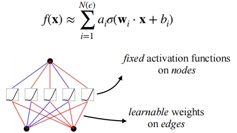
Kolmogorov-Arnold Networks (KANs), inspired by the Kolmogorov-Arnold representation theorem proposed by Russian mathematicians Andrey Kolmogorov and Vladimir Arnold in 1957, offer a groundbreaking approach to neural networks. This theorem suggests that any multivariable continuous function can be represented using a set of simpler functions.

Imagine you have a complex recipe with various ingredients and steps. The Kolmogorov-Arnold representation theorem posits that no matter how intricate the recipe, it can always be recreated using basic steps (here, basic functions). In the above equation, the input is x, and \phi_{q, p}\left(x_p\right) represents the basic univariate functions, akin to processing basic ingredients like green peppers and tomatoes. The inner summation is analogous to mixing these ingredients together. The q functions in the outer layer each take the result of the inner summation as input, and the outer summation \sum indicates that the entire function f(x) is the sum of these subfunctions q.

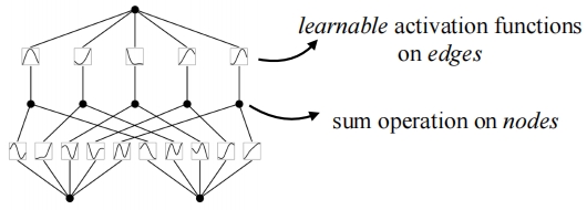
In the diagram, this is equivalent to a two-layer neural network. The key differences are, first, there is no linear combination; instead, activation is applied directly to the inputs. Second, these activation functions are not fixed but can be learned.

Compared to MLPs, which perform a unified nonlinear space transformation at each layer, this approach individually applies nonlinear transformations to each coordinate axis before combining them to form a multidimensional space.

Expressed in vector form, the equations are:

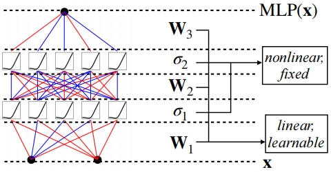
KANs do not rely on the nested relationship of activation functions and parameter matrices seen in MLPs. Instead, they involve the direct nesting of nonlinear functions, allowing for a more flexible and powerful approach to function representation.

Note: all nonlinear functions in KAN share the same structural form, controlled by different parameters.

Specifically, this study chooses splines from numerical analysis for this purpose. The term "spline" originates from a flexible spline tool used in shipbuilding and engineering drawing to create smooth, curved shapes.

The study of spline functions began in the mid-20th century, and by the 1960s, they were successfully applied to shape design through integration with computer-aided design. Since then, spline theory has evolved into a powerful tool for function approximation.

The major difference between KAN and MLP is the shift from fixed nonlinear activation functions with linear parameter learning to directly learning the parameters of the nonlinear activation functions. Due to the complexity of these parameters, learning a single spline function is inherently more challenging than learning a linear function. However, KANs typically enable smaller computation graphs than MLPs, allowing for a smaller network size to achieve the same effect. For instance, the article demonstrates that in solving partial differential equations (PDEs), a two-layer KAN with a width of 10 achieves higher accuracy (mean squared error of 10^{-7} vs. 10^{-5}) and greater parameter efficiency (100 parameters vs. 10,000) compared to a four-layer MLP with a width of 100.

You might wonder why this seemingly simple idea hasn't been widely adopted before. Indeed, they have, but previous efforts were hindered by the limitations of the original two-layer width of (2n+1) representation method and the lack of modern techniques, such as backpropagation, to train the network effectively. The significant contribution of the KAN model lies in its further simplification and generalization to arbitrary widths and depths, while also extensively demonstrating its effectiveness in AI and science through empirical experiments, showcasing both high accuracy and interpretability. This achievement is remarkable because one of the biggest challenges in deep learning is its "black box" nature, where training networks often feel like alchemy. As models grow larger, they are more likely to encounter limitations similar to those predicted by Moore's Law for chips. KANs offer a new frontier in AI, much like quantum chips promise a fundamental transformation in computing. This reworking of existing network structures using KAN signals a shift away from the limitations of Transformers and large models, encouraging a broader perspective in AI development.

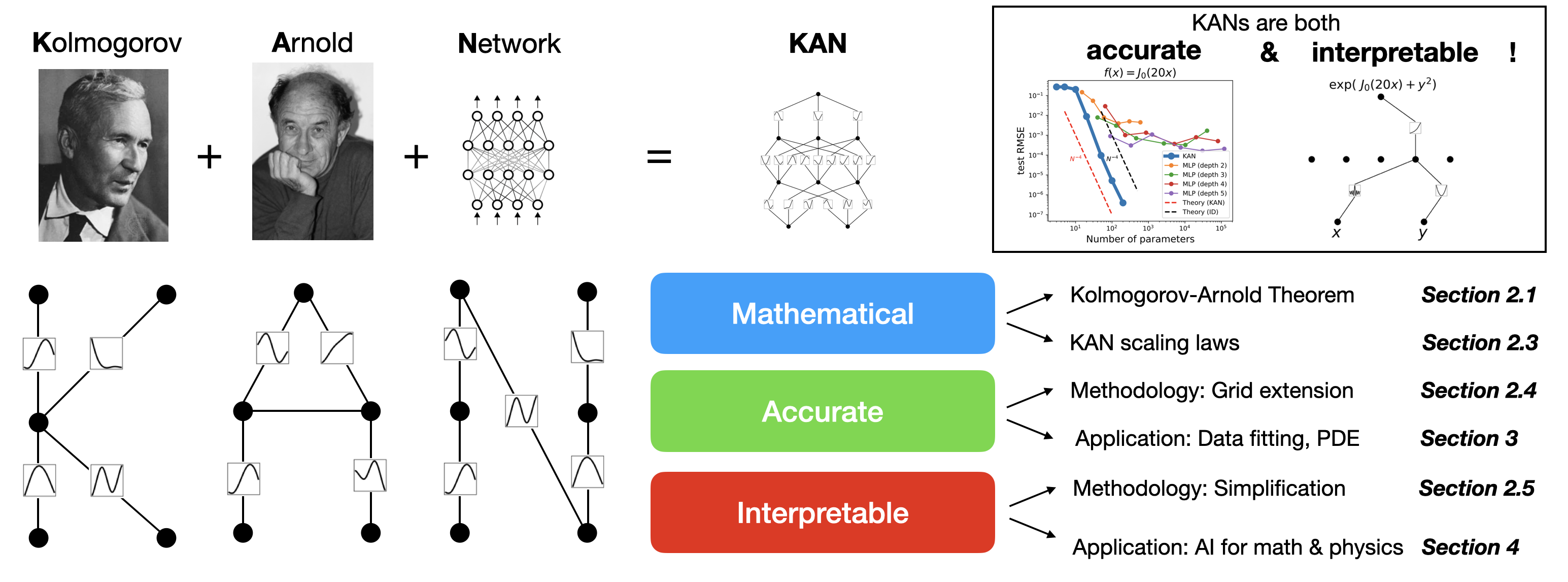
KANs are mathematically grounded, empirically validated for accuracy, and offer strong interpretability, making them a promising advancement in deep learning.

Deep Dive into the KAN Architecture

Detailed Explanation

The diagram clearly demonstrates the principle of the entire network architecture. By combining many quarter-period sine-like functions, the network can fit any function. In other words, using the B-spline activation function with two summations is sufficient to achieve this versatility.

The structure shown in the diagram utilizes a combination of two scales or resolutions: coarse-grained and fine-grained grids. This approach maintains computational efficiency while more accurately capturing and adapting to function changes. Although this basic structure is not particularly novel and has existed before, the challenge lies in deepening it. Relying solely on this approach is insufficient for approximating complex functions. Addressing this challenge and effectively deepening the architecture is the main contribution of the paper.

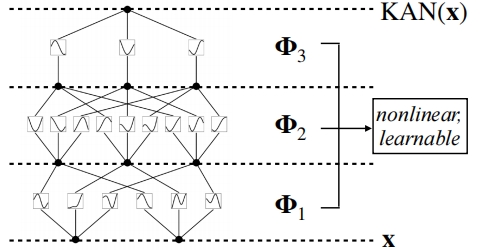
To construct a deep KAN, one must first address the fundamental question: "What constitutes a KAN layer?" Simply put, a KAN layer is a matrix of one-dimensional functions.

In this configuration, the first layer of a two-layer KAN has n inputs and 2n+1 outputs. The second layer takes these 2n+1 inputs and ultimately produces a single output. To construct a deeper network, one simply stacks more layers, similar to the approach in a Multilayer Perceptron (MLP). Essentially, this process involves determining the transition matrix between the inputs and outputs of each layer.

Here,l denotes the layer number, with the right side representing inputs and the left side representing outputs. Refer to the diagram above to understand the corresponding relationships. The input consists of 2 units, so the second layer has 2 \times 2 + 1 = 5 units. \phi represents the activation function on each edge, which is the nonlinear transformation. Essentially, each x has 5 versions, which are then combined. i labels the nodes in the current layer, and j labels the nodes in the next layer. The output of each node x_{l,i} is processed by the activation function \phi_{l,i,j} and contributes to the computation of all x_{l+1,j} in the next layer. Corresponding to the diagram, the input layer has 2 nodes, and the second layer has 5 nodes, thus the matrix is 5 \times 2. The first column of the matrix represents the 5 activation functions corresponding to x_{0,1}, and the second column corresponds to x_{0,2}, then they are combined pairwise.

Therefore, it is important to emphasize that the number of nodes in a KAN network layer is not arbitrary but determined by the number of input nodes, resulting in 2n+1 nodes. The required number of parameters or connections is (2n+1) \times n, which is significantly fewer than in a fully connected network. This reduced parameter count highlights the efficiency of KAN networks, as illustrated in the accompanying diagram.

Thus, expressing the cascading relationship of multi-layer functions in matrix form is straightforward:

Or in the expanded form:

To summarize, the original two-layer KAN network had the structure [n, 2n+1, 1]. This structure has now evolved into a multi-layer cascade, where the restriction of the 2n+1 configuration has been further relaxed, allowing the number of hidden layer nodes to be freely adjusted.

For example, in this diagram, it is clear that the number of hidden layers is not constrained to 2n+1; instead, it still involves summation at corresponding positions rather than full connection.

Implementation Details

Residual Activation Function: We include a basic function b() (similar to the function used in residual connections), so the activation function \phi(x) is the sum of the basic function b() and the spline function:

We commonly set:

Spline functions are typically parameterized as a linear combination of B-splines:

where u is trainable. In principle, u is redundant because it can be absorbed into b(x) and \text{spline}(z). However, we still include this u factor to better control the overall magnitude of the activation function. SiLU (Sigmoid Linear Unit), also known as the Swish function, is a neural network activation function first proposed in a paper by Google Brain. It gained attention for its excellent performance on certain tasks and can be considered a variant of the sigmoid function.

Assume the layers have equal width, with L layers and N nodes per layer. Each spline function typically has an order of k=3 with G intervals and G+1 grid points. "G intervals" refers to the number of segments in the piecewise definition of the spline function. Therefore, there are approximately O(N'L(G + k)) or O(N'LG) parameters in total. In comparison, a multilayer perceptron (MLP) with depth L and width N requires O(N^2L) parameters, which seems more efficient than KAN in terms of computational complexity. However, KANs typically require much smaller neural networks (NNs) than MLPs. This reduction not only saves parameters but also improves generalization and interpretability.

In other words, due to the expressive power of spline functions, KAN can achieve strong expressive capability without requiring a large number of nodes. Hence, overall, it can save a significant number of parameters compared to MLPs.

Discussion on Approximation Capability and Scaling Laws

This paper spends a page deriving and proving the theorem:

This part can be challenging to grasp, so it's normal to find it confusing. Simply put, it mathematically proves that constructing a multi-layer B-spline function network can effectively approximate complex functions. Despite increasing the network's depth and complexity, KANs can approximate high-dimensional functions through detailed grid partitioning without suffering from the curse of dimensionality. The curse of dimensionality refers to the problem of data sparsity and processing complexity increasing dramatically in high-dimensional spaces. Remarkably, the residual rate in KANs does not depend on the dimension, thus overcoming the curse of dimensionality.

Let's take a closer look at the so-called scaling laws. Note that the scaling laws discussed here differ from those in the field of large models. In large models, scaling laws suggest that as model size (e.g., the number of parameters) increases, the model's performance (such as accuracy in language tasks) typically improves, sometimes described by mathematical relationships like power laws with C = 6ND. Here, the focus is more on theoretical and mathematical analysis, discussing how performance improves with an increase in the number of parameters. This section primarily compares various theories aimed at guiding the practical design of neural networks for more efficient learning and generalization, and can mostly be skipped for now.

How to Improve Accuracy?

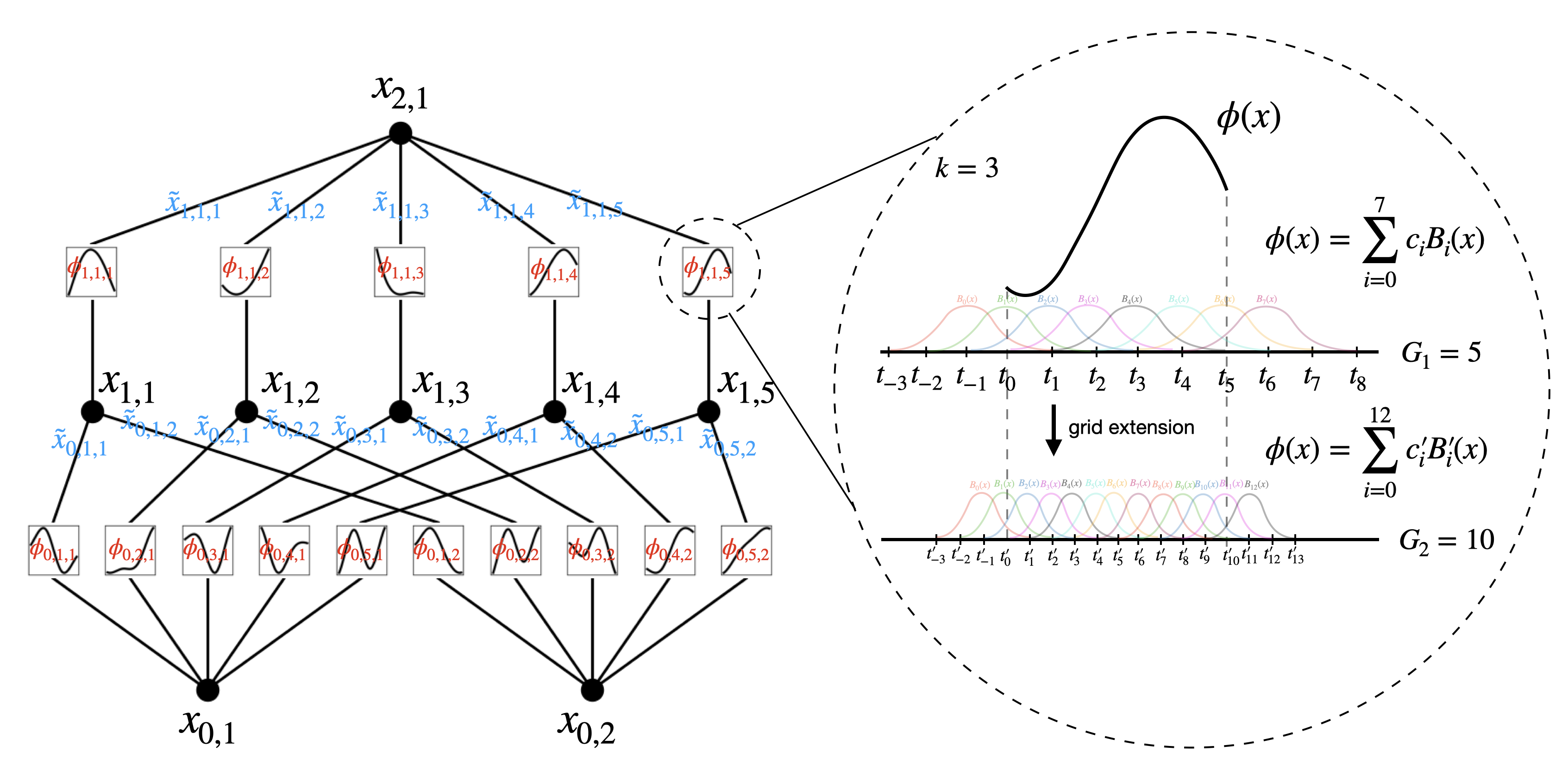
MLPs can improve performance by increasing the model's width and depth, but this approach is inefficient as it requires independently training models of different sizes. In contrast, KANs can start with fewer parameters and then increase the parameters by simply refining their spline grid, eliminating the need to retrain the entire model.

The basic principle involves expanding the existing KANs by converting the coarse grid of splines into a finer grid and correspondingly adjusting the parameters. This technique is known as "grid extension."

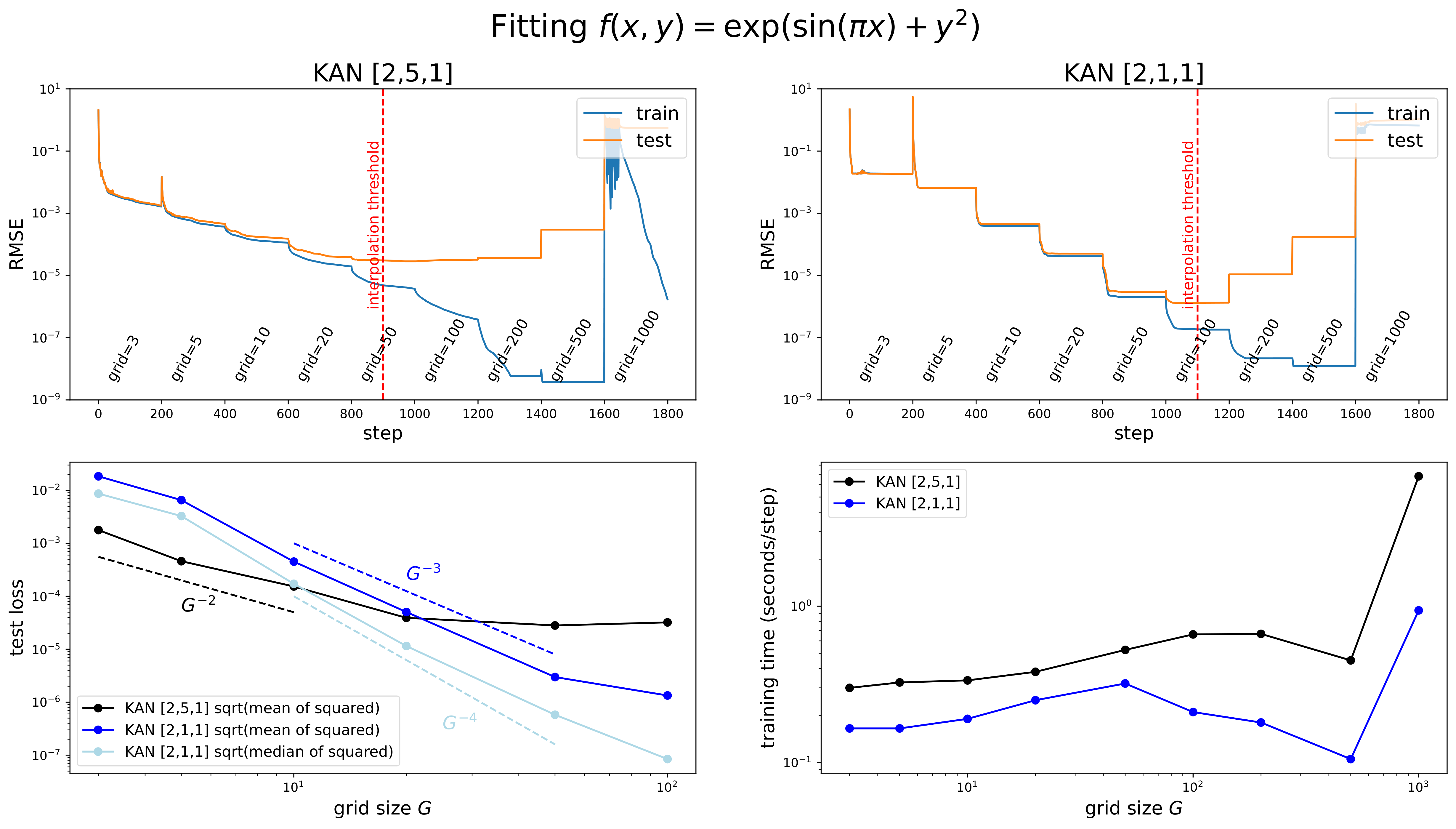
The paper uses a small example to demonstrate this point by approximating a function with KANs. In the upper diagram, each "grid-x" label on the horizontal axis represents the point at which grid refinement occurs at a specific training step. Each label indicates an increase in the number of grid points at that step, allowing the model to more finely approximate the target function, usually resulting in a decrease in error. This demonstrates that increasing the grid points directly impacts the model's learning effectiveness and improves the accuracy in approximating the target function. The left and right images represent networks of two different structures.

The two diagrams above respectively show the test error as a function of grid size (bottom left) and the training time as a function of grid size (bottom right). The conclusion is that the error (loss) exhibits different scaling relationships with grid size G at different scales. Training time increases with grid size, particularly when the grid is very large (approaching 1000), where the training time rises sharply.

These observations support the paper's claim that KANs can effectively improve accuracy through grid extension without the need to retrain the entire model. They also suggest that when selecting grid size, there is a need to balance model accuracy and training efficiency. In simple terms, an overly fine grid is not ideal as it becomes excessively time-consuming.

How to Improve Interpretability?

Despite the many benefits of KANs, designing network structures for practical problems can be somewhat enigmatic. To address this, the paper proposes a method for automatically discovering optimal network structures using sparse regularization and pruning techniques. This approach starts with larger KANs and then prunes them to enhance interpretability. The pruned KANs become easier to understand and analyze compared to their unpruned counterparts.

To maximize KANs' interpretability, the paper suggests several simplification techniques and provides an example of how users can interact with KANs to enhance their clarity. These techniques make KANs more accessible and practical for real-world applications.

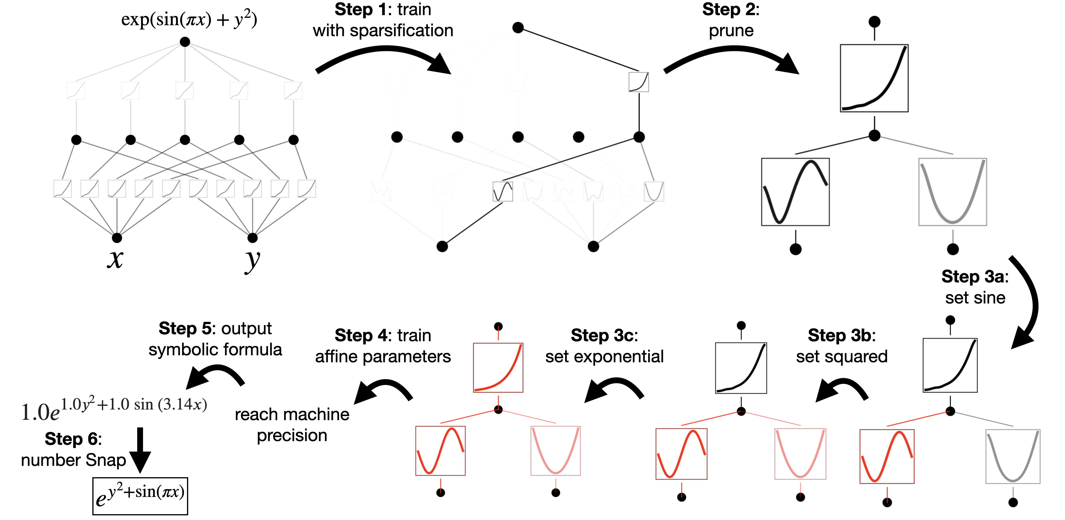
1. Sparsification: Train KANs on a dataset to fit the target function as closely as possible. MLPs typically use L1 regularization to promote weight sparsity. L1 regularization tends to shrink weight values towards zero, particularly those weights that have minimal impact on the model's output. Sparsifying the weight matrix reduces model complexity, storage requirements, and computational burden because only non-zero weights need to be processed. It also enhances the model's generalization ability and reduces the risk of overfitting.

2. Pruning: After sparsification, further remove unimportant connections and neurons through pruning techniques.

3. Setting Specific Activation Functions: Based on the characteristics of neurons after pruning, manually set or adjust specific activation functions for certain neurons.

4. Training Affine Parameters: After adjusting the activation functions, retrain the remaining parameters in the model to optimize them for the best data fit.

5. Symbolization: Finally, the model will output a symbolic formula, which approximates the original target function but is usually more concise, easier to understand, and analyze.

Experimental Validation and Results

The paper dedicates considerable space to reporting detailed simulation results, which is one of the reasons it has generated significant attention. These results primarily include accuracy and interoperability metrics.

Accuracy of KAN

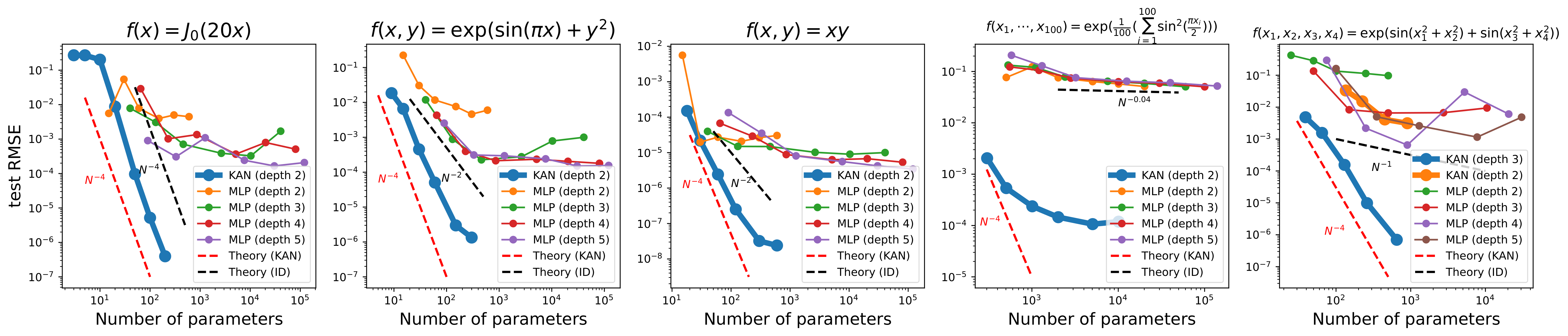
The paper compares the performance of KANs and MLPs in approximating 5 typical functions. The horizontal axis represents the number of parameters, while the vertical axis shows the root mean square error (RMSE). Overall, both KANs and MLPs exhibit a decrease in RMSE as the number of parameters increases.

In most cases, KANs (represented by the blue line) have a lower RMSE than MLPs of the same depth, particularly when the number of parameters is smaller. This suggests that KANs may have higher parameter utilization efficiency. MLPs show a slower performance improvement after a certain number of parameters, quickly reaching a plateau, possibly due to inherent limitations in fitting these types of functions. KANs closely follow or match the theoretical curve in multiple test cases.

This indicates that KANs may be a better choice for handling complex functions and high-dimensional data, offering better scalability and efficiency. This performance advantage is particularly important when learning complex patterns from limited data, such as in tasks like physical modeling, sound processing, or image processing. Although these are still relatively theoretical experimental data, they provide significant insights.

Further comparisons of KANs and MLPs on challenging special function fitting tasks yielded similar conclusions. As the number of parameters increases, KAN (blue) performs stably and continues to improve, while MLPs (yellow) reach a plateau. KANs maintain low error while demonstrating better parameter efficiency and generalization ability. This is extremely important for designing efficient and accurate machine learning models, especially in applications with limited resources or high accuracy requirements.

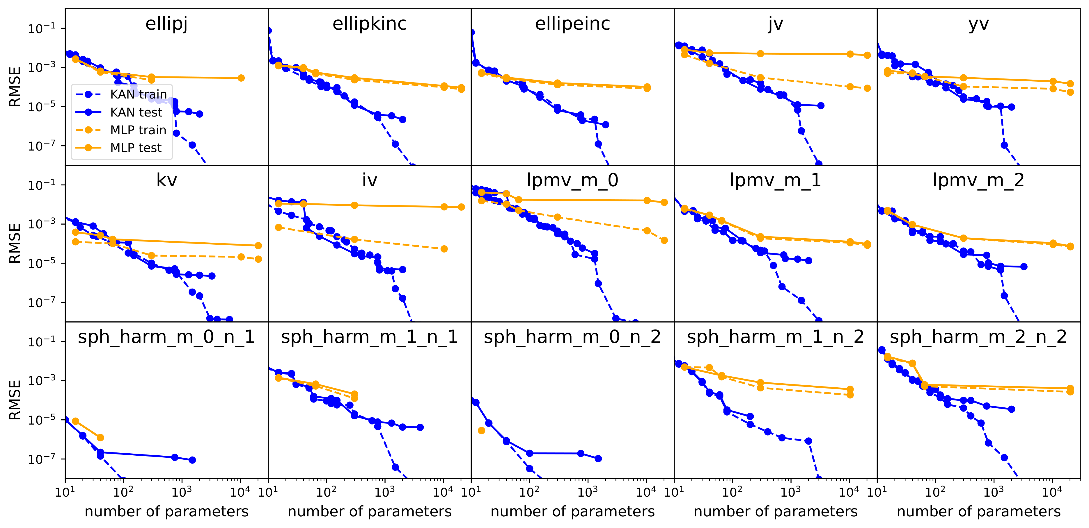
These functions involve special mathematical functions such as elliptic integrals and Bessel functions.

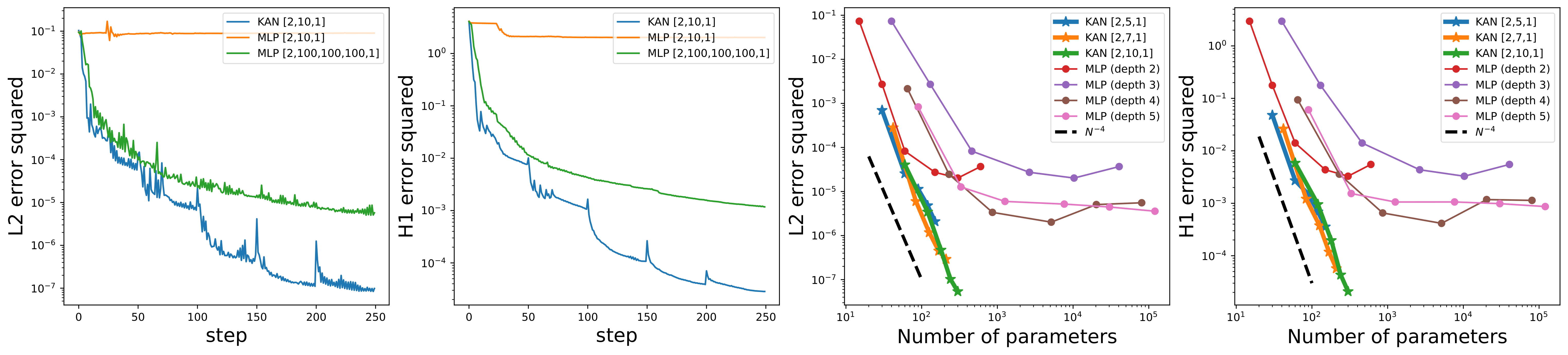
Then, examples of solving partial differential equations were provided. Compared to MLPs, KANs achieved lower errors with the same number of parameters. This demonstrates the superior efficiency and accuracy of KANs in handling complex mathematical problems, highlighting their potential as a powerful tool in various scientific and engineering applications.

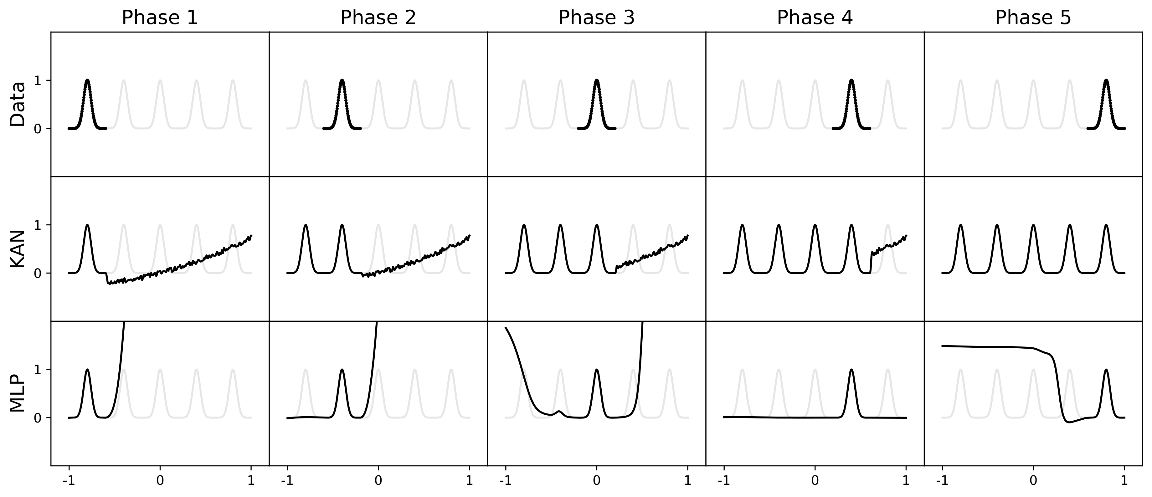
Next, the continuous learning problem was discussed. The top row shows one-dimensional data used for regression tasks, consisting of five Gaussian peaks presented sequentially, with each stage showing only a portion of the data peaks. The middle and bottom rows display the fitting results of KANs and MLPs, respectively, across five learning stages. KANs were able to retain previously learned knowledge while learning new data, whereas MLPs exhibited severe catastrophic forgetting, meaning that newly learned information significantly interfered with the memory of old knowledge.

Interpretability of KAN

Supervised Learning Example

With the help of techniques to enhance model interpretability, such as sparsification and pruning, the final network structure formed by KAN not only fits mathematical functions but also reflects the intrinsic structure of the functions being fitted.

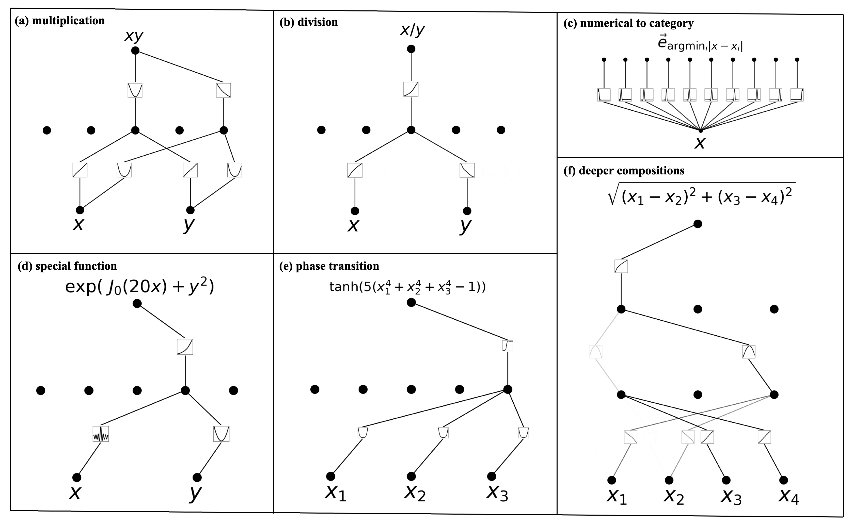
Take the first diagram as an example:

Function: f(x,y) = 2xy

Explanation: The structure in the diagram uses the identity 2xy = (x + y)^2 - x^2 - y^2 to compute multiplication. This demonstrates how KAN combines basic operations (addition, squaring) to perform complex multiplication, showing how KAN constructs more complex functions through fundamental mathematical operations.

In this example, x and y are each summed through linear functions, then squared, and simultaneously the squares of x and y are subtracted. Therefore, the impressive aspects of the KAN model are twofold: first, it's not just about the model structure itself—while MLP performs combination first and then nonlinear activation, KAN does nonlinear activation first and then combination; second, KAN's training can optimize its structure, giving it a somewhat self-organizing nature.

Unsupervised Learning Example

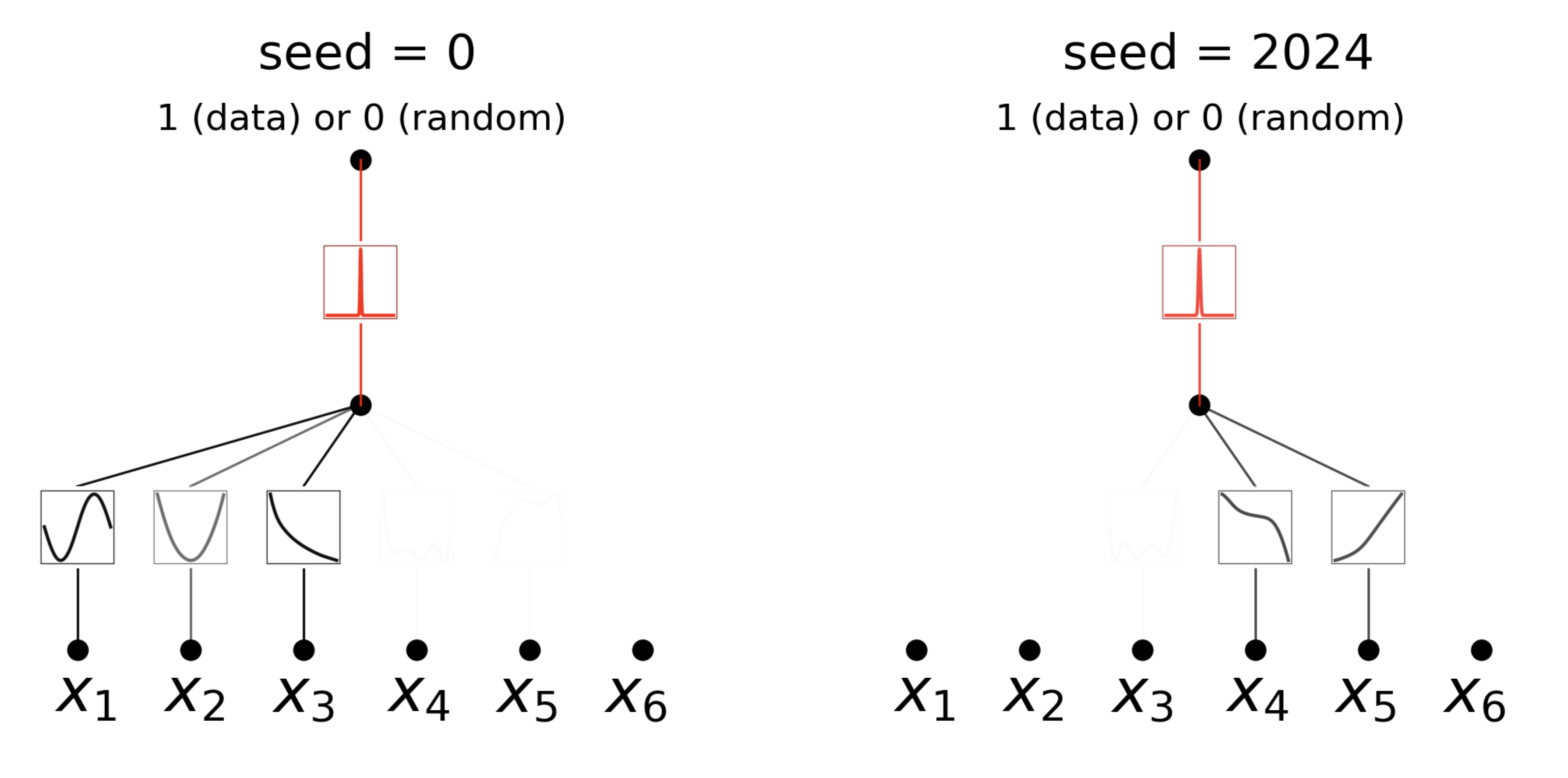
In unsupervised learning, the goal is to identify dependencies between variables in the data rather than predicting an output. By modifying its structure, KANs can identify which input variables are interdependent. The left diagram (seed=0) and the right diagram (seed=2024) demonstrate how the same dataset, but different initialization seeds, can lead KAN to learn different dependency structures.

KAN provides a powerful tool to explore these relationships through its flexible network structure, thereby enhancing the interpretability and broad applicability of the model.

Mathematical Applications

Using KANs to address problems in Knot Theory, which is a branch of topology that studies mathematical knots. Diagram (a) shows a network structure using 17 variables, achieving 81.6% test accuracy. A simplified model using only the 3 most important variables achieved 78.2% test accuracy. Diagram (c) presents a pie chart displaying the contribution proportions of the three variables to the prediction results.

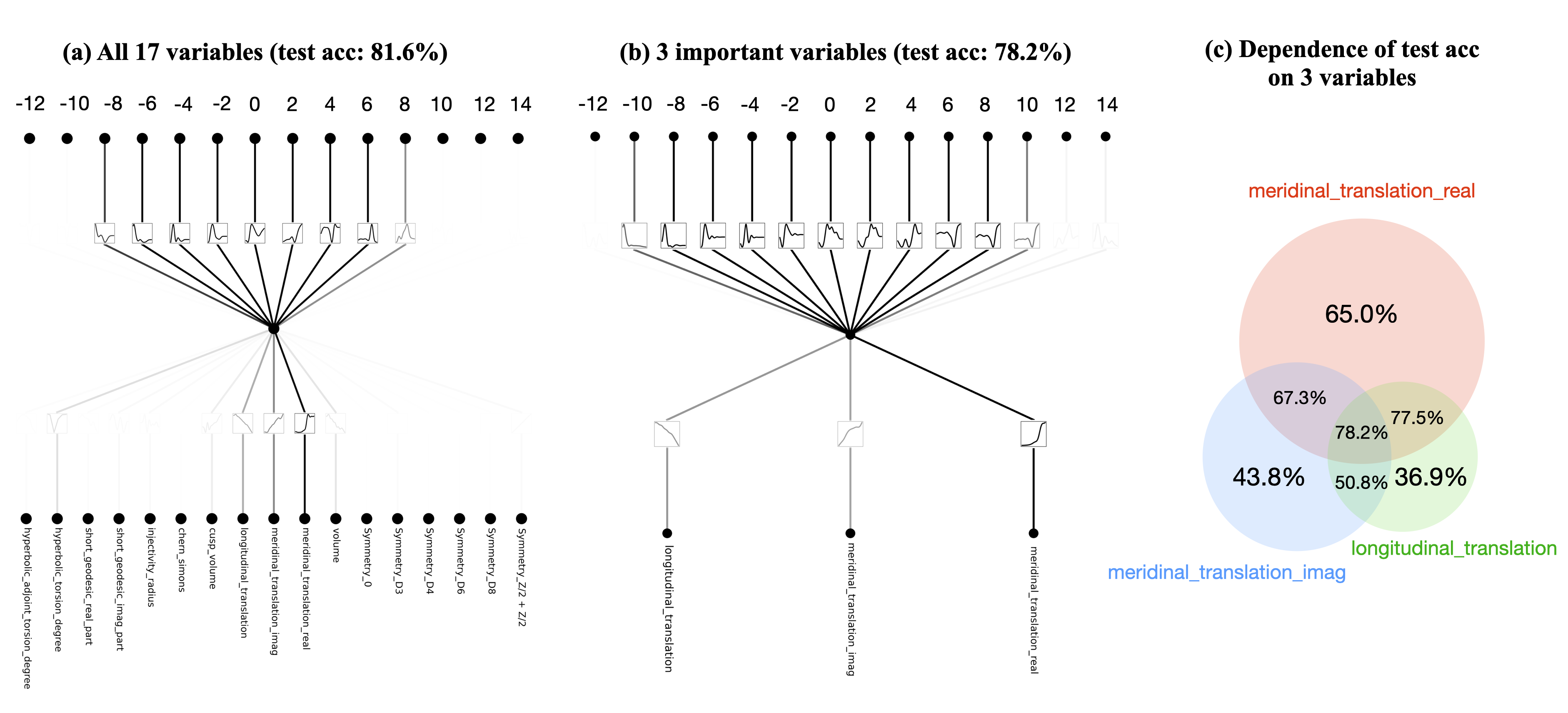
By optimizing the selection of input variables, KANs can significantly reduce model complexity while maintaining high accuracy. This is particularly important for applications that aim to reduce computational resource consumption while improving model interpretability. In other words, KAN's training algorithm can achieve self-selection and optimization of the network structure to some extent.

If the above example is still supervised learning and can only be used for validation, then in unsupervised learning, KANs can also be used to discover new data structures. This capability is demonstrated in the following example:

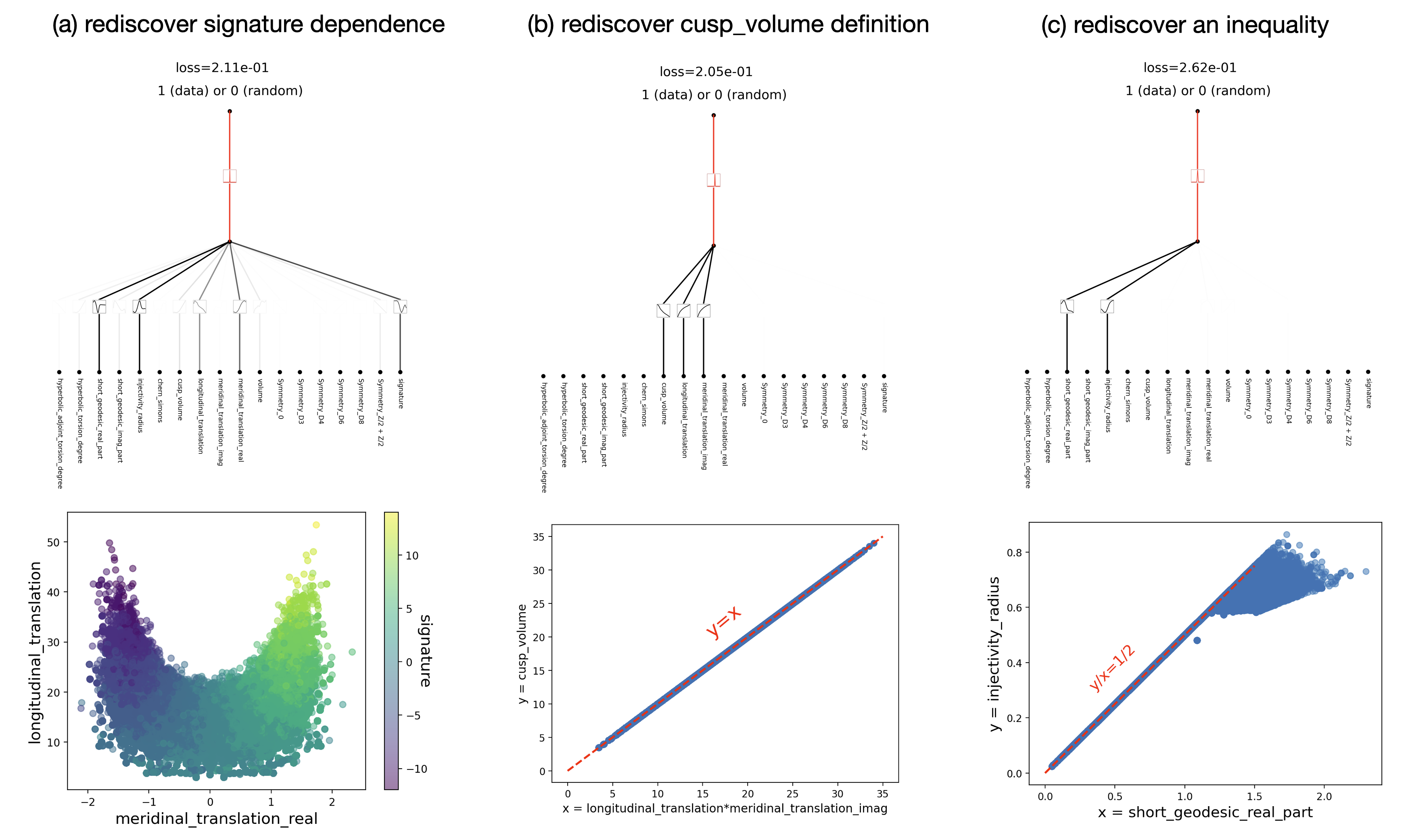
Diagram (a) rediscovered signature dependencies, while Diagram (b) demonstrates how KANs can rediscover the definition of cusp volume through a self-learning process without any prior knowledge. In Diagram (c), data points are distributed around the line y = \frac{x}{2}, indicating a direct linear relationship between y and x. y is always less than or equal to half of x, essentially rediscovering an inequality. This self-discovery ability illustrates that KANs can serve as a powerful tool for exploring hidden patterns in data.

Physical Applications

Next, the paper continues to use KANs to explore and interpret dynamical boundaries in physical models, particularly in the application of the Anderson localization phenomenon in quantum systems.

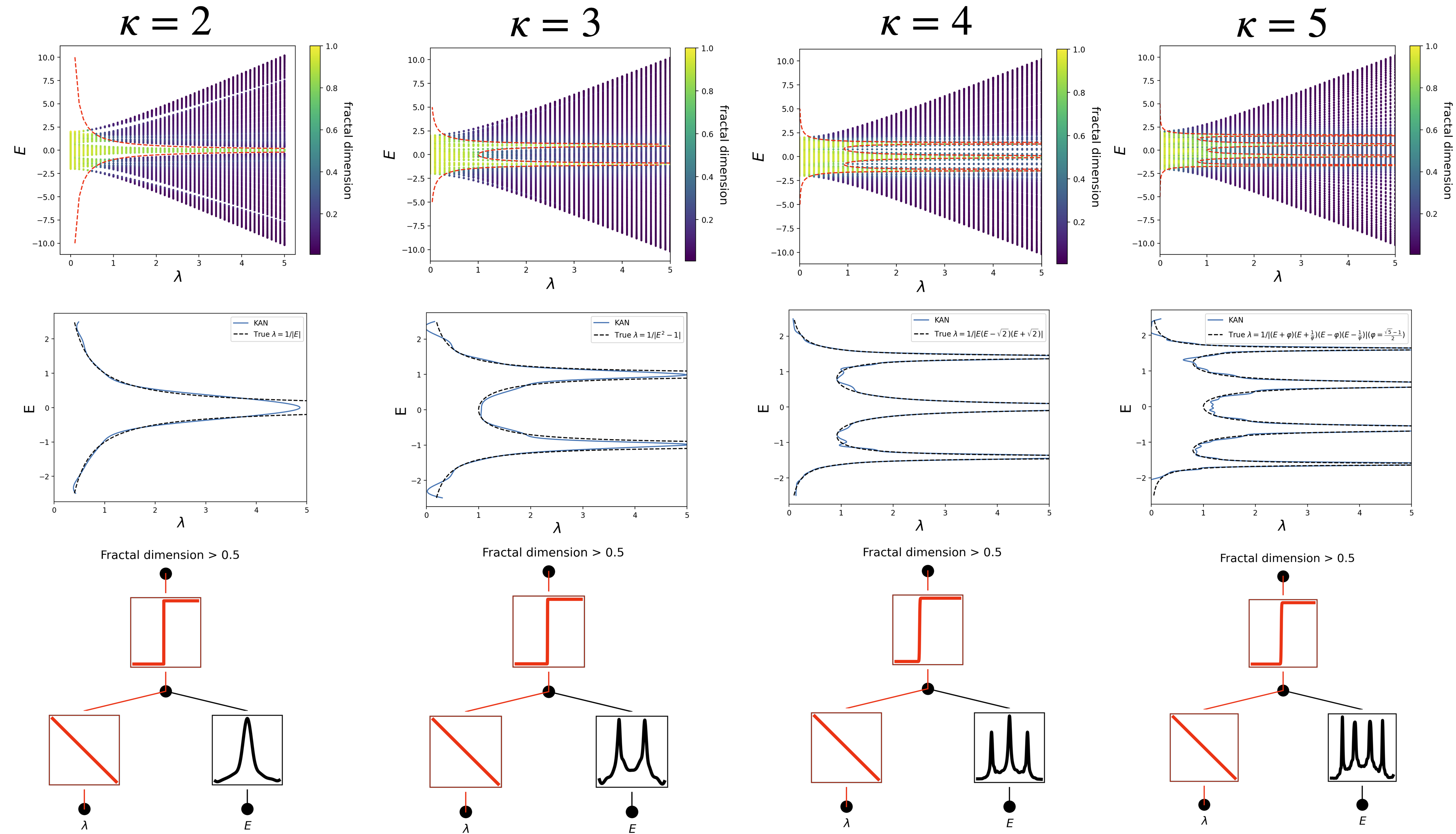
This diagram shows the application of KANs to two specific physical models.

Top: Displays the phase diagram of the model, depicting the physical states under varying system parameters.

Middle: Shows the behavior of the system's characteristic size with changes in system parameters, helping to quantify the degree of localization of electronic states. The exact details are also not essential for us to understand.

Bottom: Provides the corresponding KANs structure, showing how the network learns to output corresponding physical behavior (such as localization states) from input data (system parameters) and highlights the key network nodes and connections. This helps to understand the most important physical quantities in the model, aiding in comprehension.

Since KANs training can automatically select the structure and the structure can have some physical significance, can this structural optimization be controlled manually? The article then provides an example comparing automatic and manual modes:

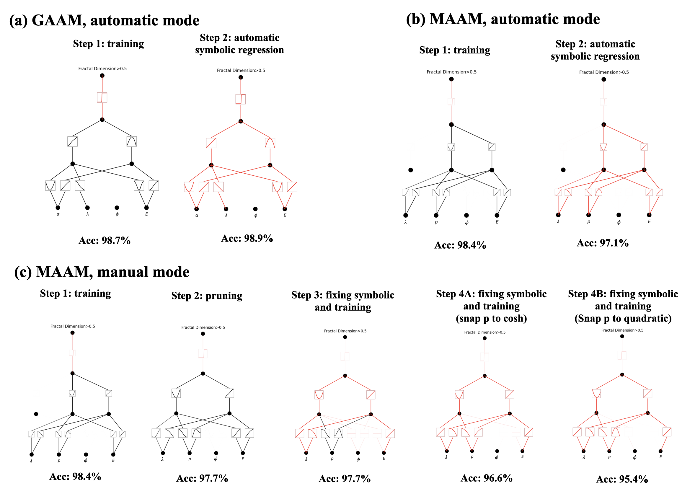
In automatic mode, KANs completely construct and optimize the network structure based on data without human intervention. This allows for quickly obtaining a working model but may lack in-depth customization for complex problems. In manual mode, users can engage more deeply in the model-building process, such as by manually setting network layers and activation functions to explore specific features or relationships in the data. Although this approach is more time-consuming, it allows for more precise adjustment of the model to fit specific scientific problems. By combining KANs' automation capabilities with users' expertise, key phenomena in physical systems can be effectively uncovered and interpreted, especially when dealing with complex systems that are difficult to analyze using traditional methods.

MLP vs. KAN: How to Make the Right Choice?

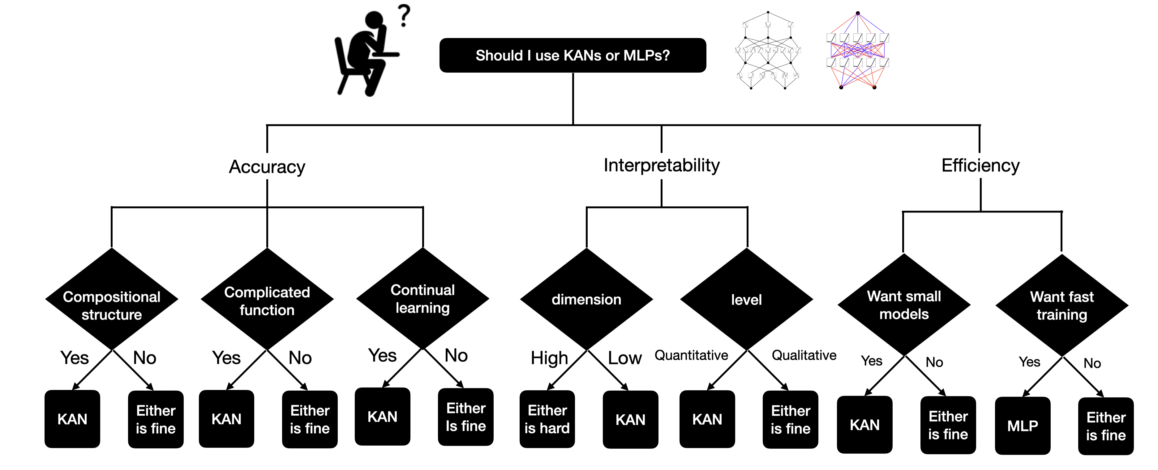
Regarding this question, the choice mainly depends on the desired outcome. If efficiency is the priority, as in the rightmost branch, then MLP is the preferred option. Currently, the training speed of KANs is its main bottleneck, typically being 10 times slower than MLPs. However, if a smaller model is preferred, KAN is better. If interpretability is the priority, the middle option, then KAN is superior. If accuracy is the priority, the leftmost option, KAN is also superior.

Despite showing promising prospects, KAN is still in its early stages and has many limitations. These include:

• Mathematics: The Kolmogorov-Arnold representation theorem has been greatly simplified, and this theorem itself does not consider deep scenarios. Incorporating the concept of depth could strengthen the mathematical foundation.

• Algorithms: The architecture design and training methods for KANs have not been fully explored to improve model accuracy. For example, replacing the spline activation function might yield better results.

• Efficiency: There is still room for improvement. Additionally, it might be worth considering whether KANs can be combined with MLPs for better performance.

Implementing KAN: A Guide to the Code

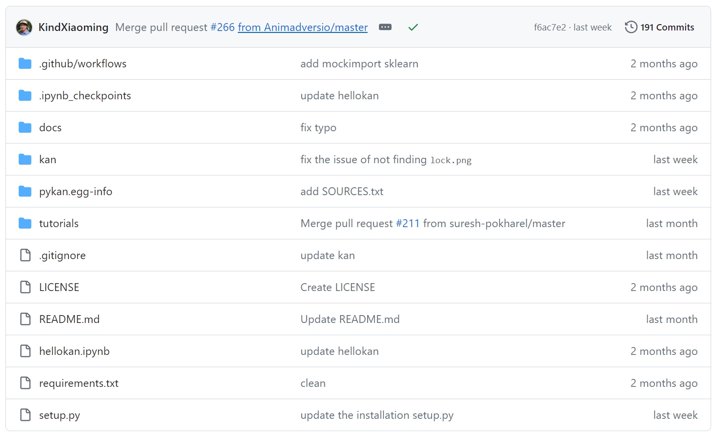
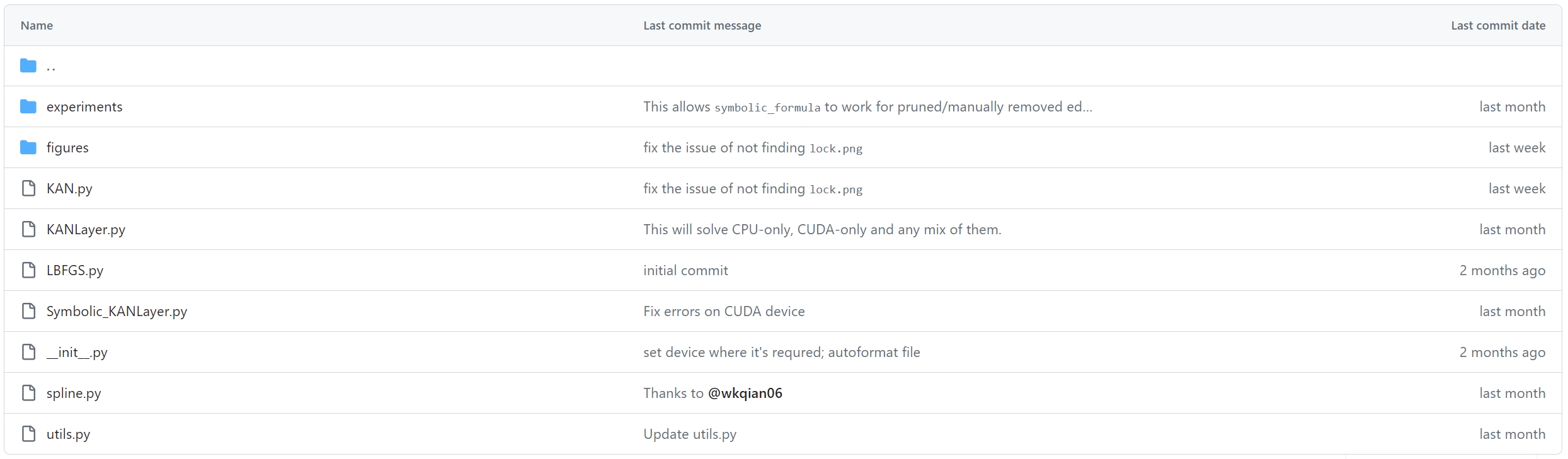
Open the code folder; the directory structure is very simple.

• KAN.py is the main file, containing the primary class or functions that define the KAN model and handle the model building and training process.

• KANLayer.py defines the custom layers used in the KAN model, including core components of the model such as special activation layers or other processing layers, which form the foundation of KAN.

• L-BFGS.py includes the implementation of the L-BFGS optimizer suitable for training KANs.

• Symbolic_KANLayer.py implements a special KAN layer for handling symbolic computations or enhancing the interpretability of the model, converting data or activation functions into symbolic forms for deeper analysis or interpretation.

• spline.py contains the code for implementing spline functions.

Let's focus on the KAN.py and KANLayer.py files. The KAN.py file defines a KAN class, which inherits from torch.nn.Module, primarily used to implement a convolution-based neural network model.

KAN Class

Attributes

• biases: A list of biases defined using nn.Linear().

• act_fun: A list of activation function layers defined using KANLayer.

• depth: The depth of the network.

• width: The number of neurons in each layer.

• grid: The number of grid intervals.

• k: The degree of the piecewise polynomial.

• base_fun: The base function used to define the basic form of the activation function.

• symbolic_fun: A list of symbolic activation function layers defined using Symbolic_KANLayer.

• symbolic_enabled: A flag to control whether the symbolic frontend is calculated to save time.

Methods

• __init__(): Initializes the KAN model, allowing the setting of network width, number of grids, polynomial degree, sound ratio, base function, etc.

• forward(): The forward propagation function, which computes the output through the network based on input data.

• train(): Trains the model, including setting the optimizer, loss function, regularization methods, etc.

• prune(): Prunes the model by removing unimportant connections or nodes to simplify the model and reduce computational load.

• plot(): Plots the network structure, showing detailed information about the connections and activation functions of each layer.

• symbolic_formula(): Extracts and returns the symbolic expression of the network, used for analyzing the mathematical structure of the network.

Code Logic Flow

1. Initialization: Initialize the network structure in the class constructor, including the setup of layers and the initialization of activation functions.

2. Forward Propagation: Define the forward propagation logic, detailing how to compute the output through each layer and activation function.

3. Training Process: Set training parameters and execute the training loop, including forward propagation, loss calculation, backpropagation, and parameter updates.

4. Pruning and Visualization: Provide methods for pruning the network and visualizing the network structure to facilitate analysis and optimization.

5. Symbolic Expression Extraction: Extract the mathematical symbolic expression of the network to deeply understand the network's working principles.

Summary and Future Directions

1. Flaws of MLP: Multilayer Perceptrons (MLPs) rely on the core principle of linear combination plus nonlinear activation. However, in deep networks, the consecutive multiplication of derivatives during backpropagation leads to issues such as gradient vanishing and explosion. Additionally, fully connected networks result in low parameter efficiency.

2. Principle of KAN: KANs use parameterized, learnable nonlinear activation functions within a single architecture to achieve nonlinear space transformations. This greatly enhances the model's representational capacity, offering a more robust alternative to traditional MLPs.

3. KAN Training Algorithm: KANs improve accuracy and interpretability through grid extension (increasing activation function resolution), sparsification, pruning, and other structural self-optimization techniques. These methods allow KANs to achieve the same or better fitting results with significantly fewer parameters compared to MLPs.

4. Experimental Validation: Simulation experiments provide quantitative evidence supporting the effectiveness of KANs. While the research is still preliminary, it indicates a promising new direction for deep learning.

The theory of deep learning has remained largely unchanged for over a decade, similar to the long-standing dominance of brick-and-mortar structures in architecture. The advent of reinforced concrete revolutionized construction, and KANs have the potential to similarly transform deep learning. By offering a new, vast blue ocean for artificial intelligence, KANs excite researchers with the possibility of revisiting and re-implementing old ideas using this innovative structure.